Geology of New Zealand Field Trip Guidebook - ResearchGate
Geology of New Zealand Field Trip Guidebook - ResearchGate
Geology of New Zealand Field Trip Guidebook - ResearchGate

Create successful ePaper yourself
Turn your PDF publications into a flip-book with our unique Google optimized e-Paper software.
HWS/U 2008<br />
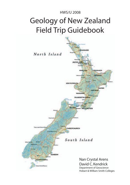
<strong>Geology</strong> <strong>of</strong> <strong>New</strong> <strong>Zealand</strong><br />
<strong>Field</strong> <strong>Trip</strong> <strong>Guidebook</strong><br />
Nan Crystal Arens<br />
David C. Kendrick<br />
Department <strong>of</strong> Geoscience<br />
Hobart & William Smith Colleges
Hobart & William Smith Colleges and Union College<br />
2008 <strong>New</strong> <strong>Zealand</strong> <strong>Guidebook</strong><br />
Nan Crystal Arens and David C. Kendrick<br />
Please read this guidebook before you arrive in <strong>New</strong> <strong>Zealand</strong><br />
Tell your parents that they can get a PDF copy <strong>of</strong> the guidebook on the web site.<br />
Bring the guidebook with you on the trip.<br />
NOTE: There is a NZ$25 fee to exit <strong>New</strong> <strong>Zealand</strong>. You will pay this after obtaining your<br />
boarding pass as you prepare to leave the country. Please budget accordingly.<br />
Itinerary<br />
13 Nov. Arrive in <strong>New</strong> <strong>Zealand</strong>, store bags and transit to Christchurch<br />
14 Nov. Meet group 9 a.m. for drive to Aoraki<br />
15 Nov. Mueller and Hooker Glacier Moraines—<strong>Field</strong> Exercise<br />
16 Nov. Travel through Haast Pass to Haast Beach<br />
17 Nov. Alpine Fault and travel to Franz Josef<br />
18 Nov. Franz Joseph Glacier<br />
19 Nov. Travel to Arthur’s Pass<br />
20 Nov. Travel to Christchurch (free evening)<br />
21 Nov. 6:45 a.m. flight to Wellington and travel to National Park<br />
22 Nov. Tongariro Crossing or Ruapehu or field exercise<br />
23 Nov. Tongariro Crossing or Ruapehu or field exercise<br />
24 Nov. Tongariro Crossing or Ruapehu or field exercise<br />
25 Nov. Travel to Rotorua and Waimangu geothermal field<br />
26 Nov. Wai-o-tapu geothermal field<br />
27 Nov. White Island and Maori Thanksgiving Feast<br />
28 Nov. Final exam and call home (it’s Thanksgiving in the States)<br />
29 Nov. Program ends. Transit to Auckland for departing flights.<br />
Contact Information<br />
Pr<strong>of</strong>. Nan Crystal Arens arens@hws.edu<br />
Pr<strong>of</strong>. David C. Kendrick kendrick@hws.edu<br />
Center for Global Education cge@hws.edu, 315-781-3807 (emergency 315-781-2387)<br />
Mobile phone information for Pr<strong>of</strong>s. Arens and Kendrick will be posted on the program web<br />
site (http://academic.hws.edu/Kendrick/OZ2008) as soon as it is available. This site should<br />
also be consulted for any changes in itinerary and important notices.<br />
Because we are almost constantly on the move during the <strong>New</strong> <strong>Zealand</strong> field trip, it may be<br />
difficult for family and friends to contact you. Furthermore, we will be in some relatively<br />
remote areas where internet access may not be available or only available through a very<br />
slow dial-up connection that may be incompatible with the HWS and Union mail servers.<br />
Where internet access is available, it will likely be on a pay-for-time basis (~NZ$5 for 10-15<br />
minutes). You should plan ahead to call home. Phone cards with reasonable international<br />
rates can be purchased throughout <strong>New</strong> <strong>Zealand</strong>. In an emergency, family and friends should<br />
try first to contact Pr<strong>of</strong>s. Kendrick or Arens using the mobile numbers provided on the web<br />
site (http://academic.hws.edu/Kendrick/OZ2008). Please note, however, that mobile<br />
1
coverage is not available in all areas we will visit. Failing to reach the program directors,<br />
emergency messages can be relayed through the Center for Global Education. We have also<br />
provided contact information for each <strong>of</strong> the places we will be staying (see page 3).<br />
Important Schedule Notes<br />
Arrival in Auckland 13 November—Your flight to <strong>New</strong> <strong>Zealand</strong> should route you through<br />
Auckland, <strong>New</strong> <strong>Zealand</strong>’s capital and the city from which the group flight departs at the end<br />
<strong>of</strong> the program. You must store your luggage, except for one bag and a day-pack. We will<br />
be traveling on small-ish busses that do not have luggage space for extra bags. You have<br />
several options for luggage storage. There is a bag storage facility in the international<br />
terminal with which we have negotiated a half-price rate <strong>of</strong> NZ$110/bag for 17 days (the<br />
duration <strong>of</strong> the trip). Mention David Kendrick’s name and the HWS/U Program when you<br />
check in. There are also public lockers in the international terminal. Small lockers are<br />
90x42x55 cm for NZ$15/day. Large lockers are 90x42x87 cm for NZ$20/day. You might<br />
economize by sharing a locker <strong>of</strong> you can cram your bags in and are arriving and departing<br />
together. There are no lockers in the domestic terminal although there are a few small<br />
lockers available in the visitor’s center near the airport. These are commonly full, but you<br />
are welcome to check them out if these options do not appeal to you.<br />
Arrival in Christchurch 13 November—The group ticket you purchased will include a<br />
domestic flight to Christchurch on the afternoon/evening <strong>of</strong> 13 November. Once you arrive<br />
in Christchurch, you are responsible for your own supper and hostelry on the night <strong>of</strong> 13<br />
November and breakfast the next morning.<br />
<strong>Field</strong> <strong>Trip</strong> Departure 14 November—The program will rendezvous at 9 a.m. on Friday 14<br />
November in Latimer Square to depart for the field trip. Assemble on the corner <strong>of</strong><br />
Hereford and Latimer streets near the Kukul Kwan Korean restaurant. The coach will be<br />
waiting there for us. There are a number <strong>of</strong> backpacker type accommodations near the park.<br />
Program End 29 November—The program will formally end following the final exam on<br />
Friday 28 November. The program will provide breakfast for you the morning <strong>of</strong> 29<br />
November and the bus will depart for the Auckland International Airport following breakfast<br />
if you wish to travel back to Auckland. You are responsible for all arrangements from this<br />
point on. You are welcome to depart the program any time after the final exam.<br />
About the <strong>Guidebook</strong><br />
Please refer to the program web site (http://academic.hws.edu/Kendrick/OZ2008) for the<br />
most up to date information. While we have made every effort to ensure that all the logistic<br />
information in the guidebook is accurate, the guidebook was prepared in advance and<br />
sometimes things change. We will do our best to keep you updated, but check the website if<br />
you’re in doubt. We’ll make every effort to keep it up to date.<br />
This guidebook is an informal publication designed to help you gain a deeper appreciation for<br />
the places we will visit and to provide helpful background. We are indebted to John Garver<br />
<strong>of</strong> Union College and Brooks McKinney <strong>of</strong> HWS for much <strong>of</strong> the information herein.<br />
Information in the guidebook has been assembled from a wide variety <strong>of</strong> sources, most <strong>of</strong><br />
which have not been formally documented for you. Where we have found particularly useful<br />
references, they are noted.<br />
2
Overnight Accommodation Information<br />
November 14-15<br />
Chalets at the Hermitage—Aoraki/Mount Cook National Park<br />
www.mount-cook.com<br />
+64-3-435-1809<br />
November 16<br />
Haast Beach Holiday Park—Haast Beach<br />
+64-3-750-0860<br />
November 17-18<br />
Mountain View Top 10—Franz Josef<br />
+64-3-752-0735<br />
19 November<br />
Mountain House Backpackers—Arthur’s Pass<br />
www.trampers.co.nz<br />
+64-3-318-9258<br />
20 November<br />
North South Holiday Park—Christchurch<br />
www.northsouth.co.nz<br />
+64-3-359-5993<br />
21-24 November<br />
Discovery Lodge—National Park<br />
www.discovery.net.nz<br />
+64-0800-122-122<br />
25-28 November<br />
Kiwipaka—Rotorua<br />
www.kiwipaka-yha.co.nz/rotorua/rotorua.html<br />
+64-7-347-0931<br />
3
Gear for the <strong>New</strong> <strong>Zealand</strong> <strong>Trip</strong><br />
For the <strong>New</strong> <strong>Zealand</strong> field trip you will not need any “evening out” types <strong>of</strong> clothes, lots <strong>of</strong><br />
shoes etc. We will be outside for at least part <strong>of</strong> every day and some days we will be on long,<br />
all-day hikes in rough terrain. Our field work will go on regardless <strong>of</strong> weather, so you must<br />
be prepared for wet weather, cold weather, windy weather, intense sun and any combination<br />
<strong>of</strong> these. Several places that we will stay have laundry facilities, so you will be able to wash<br />
clothes during the trip. Do not bring too much stuff!<br />
Day pack big enough for lunch, rain gear, water and a sweater or fleece<br />
<strong>Field</strong> notebook<br />
<strong>Field</strong> trip guidebook<br />
Passport, tickets, travel documents<br />
Pens and pencils<br />
Hand lens if you have one<br />
Camera, film or memory card, charger, plug adaptor (same as in OZ), extra batteries<br />
Water bottles (minimum 2L)<br />
Hiking boots<br />
Sneakers or other close-toed shoes<br />
Sunglasses<br />
Sun hat or baseball cap<br />
Lip balm with sunscreen<br />
Sunscreen<br />
Watch for keeping track <strong>of</strong> rendezvous times when you are exploring on your own<br />
Sleeping bag<br />
Rain jacket with hood, rain pants (recommended) It will rain and we will be out in it!<br />
Gloves, winter hat<br />
Heavy sweater or fleece to layer under rain jacket<br />
2 pairs <strong>of</strong> long pants<br />
1-2 pairs <strong>of</strong> shorts<br />
At least one long sleeve shirt<br />
T-shirts for about a week<br />
7-10 days <strong>of</strong> underwear<br />
Hiking and sneaker socks<br />
Sleepwear (we will be in backpackers and other shared accommodations)<br />
Towel<br />
Toiletries<br />
Medication and other personal supplies<br />
Flashlight<br />
Casual reading<br />
Music player and headphones<br />
Personal goodies (cards, musical instruments, knitting, hacky sack etc.)<br />
Computer? You will not need your computer for course work<br />
4
What to do in an earthquake?<br />
Drop, take cover and hold. Move only a few meters to a safer place. Stay indoors until the<br />
shaking stops and you are sure it is safe to go outside. Stay away from windows, chimneys,<br />
and shelves with heavy objects. If you are in bed, stay there, put the pillow and blanket over<br />
your head to protect it from falling debris. If you are outside, drop to the ground in a clear<br />
spot away from buildings and power lines. If you are in a car, pull over and stay in the car.<br />
If you are in an elevator, stop at the nearest floor and get out. Be prepared! Keep your shoes<br />
and a flashlight within easy reach <strong>of</strong> your bed. Identify two possible exits before you go to<br />
bed. After the shaking stops, be alert to fire hazards and downed electrical lines. Expect<br />
aftershocks that may be as intense as the main event. If you are traveling with a group,<br />
gather together and move to a safe place.<br />
<strong>Field</strong> Book Assignments<br />
Here are the point values for the field book work:<br />
Date Location Points<br />
14 – 15 Nov Aoraki 20<br />
17 Nov Knights Point, Monro Beach, Fox Glacier, Alpine Fault 15<br />
18 Nov Franz Josef 15<br />
20 Nov Arthurs Pass, Castle Hill, Torlesse Pullout 10<br />
22-24 Nov National Park Fence Diagram 20<br />
25 Nov Five Mile Bay, Wairaikei Geothermal Plant, Waimangu 15<br />
26 Nov Wai-o-tapu 15<br />
27 Nov White Island 10<br />
5
Guidelines for <strong>Field</strong> Notes<br />
There are two general elements to field notes: (1) observations and (2) interpretations.<br />
Observations are the details <strong>of</strong> where you went and what you saw while you were there.<br />
Interpretations describe what those observations tell you about the history those rocks<br />
represent.<br />
Your field notes should emphasize observation. While we’re in the field, take detailed notes<br />
on your own observations. We will be pointing things out along the way and discussing what<br />
it might mean, but those discussions won’t cover everything. Although it is worthwhile to<br />
note what we say, this will not give you the whole story or full marks on field notes. Get in<br />
the habit <strong>of</strong> noting down the same set <strong>of</strong> observations at each stop.<br />
At any field site, you should include the following information in your notes:<br />
• Date, time, and weather conditions<br />
• Name the stop. If there is some name already attached, use it. If not, choose<br />
something informative.<br />
• Where is it? Include GPS coordinates if they’re available. What cities, towns or<br />
parks are nearby? Is it by the side <strong>of</strong> the road? Etc.<br />
• What is the landscape like? Describe the topography. Describe the outcrop itself and<br />
include a map and a sketch. They don’t have to be artist-quality, just something that<br />
conveys what it looks like. Make sure you include a scale and the orientation (i.e.,<br />
which way is north).<br />
• Geologic context. If you know the formation names, include them. Likewise include<br />
the age, if you know.<br />
• What types <strong>of</strong> rocks are present? Provide detailed descriptions based on your<br />
own observations. Do this in a systematic way. See the section below for<br />
suggestions on rock descriptions.<br />
• Are fossils present? If there aren’t any say so. If there are, note what they are.<br />
Describe them. Drawings are even better. Make sure to include a scale.<br />
• What structural features do you observe? Are the beds horizontal? Tilted? Are there<br />
faults, folds, or joints? What are their orientations?<br />
• What events do you observe? Are there beds? Are they all the same? If not, how are<br />
they different? Are there changes in sedimentation style? Can you see any cyclicity<br />
(repetitions)? Evidence <strong>of</strong> volcanic activity? Metamorphism? Faulting and folding?<br />
Can you tell the order <strong>of</strong> events? Something else?<br />
• Anything else you deem interesting.<br />
Rock Descriptions<br />
What to say about the rocks? Developing a systematic checklist or outline to follow when<br />
you describe a rock gives you a routine to follow each time. Establishing a routine moves the<br />
effort out <strong>of</strong> the overwhelming category and into the okay, not so hard category. Here are<br />
some guidelines. Obviously some categories will apply to some kinds <strong>of</strong> rock and not to<br />
6
others. NOTE—THESE LISTS ARE NOT EXHAUSTIVE—THEY ARE GUIDELINES<br />
FOR THE KINDS OF THINGS YOU SHOULD LOOK FOR, BUT BE ALERT FOR THE<br />
UNUSUAL. DETAIL IS IMPORTANT.<br />
• Rock type: Decide if the rock is sedimentary, igneous, or metamorphic.<br />
o Igneous – rock name, color, texture (crystal size), mineral composition,<br />
presence or absence <strong>of</strong> vesicles (bubbles), deformation <strong>of</strong> clasts (like squished<br />
or distorted pumice in ignimbrite), presence <strong>of</strong> volcanic glass, layering or<br />
other features in tephra, variation in outcrop scale, weathering.<br />
o Sedimentary – Is it clastic or chemical? Rock name, color, weathering, mineral<br />
composition, texture (grain size, sorting, and rounding), sedimentary<br />
structures (layers and their thicknesses, nature <strong>of</strong> contacts, e.g., flat, bumpy,<br />
hummocky, etc., presence <strong>of</strong> ripples, cross-bedding, etc). Are there fossils? If<br />
so, what kinds? How common?<br />
o Metamorphic – Rock name, color, texture (crystal size, crystal orientation),<br />
mineral composition, foliation, variation on outcrop scale.<br />
Some igneous rocks<br />
Phaneritic Rocks: Coarse-grained rocks with easy to see mineral grains<br />
Quartz Content Other Minerals Rock Name<br />
Quartz > 10%<br />
Orthoclase >>Plagioclase<br />
Plagioclase >= Orthoclase<br />
GRANITE<br />
GRANODIORITE<br />
% Dark Minerals < 25% SYENITE<br />
Quartz < 10%<br />
% Dark Minerals 25-50% DIORITE<br />
% Dark Minerals > 50% GABBRO<br />
Aphanitic Rocks: Fine-grained rocks where only a few mineral grains are large enough to be<br />
easily seen (phenocrysts)<br />
Rock color Phenocryst Minerals Rock Name<br />
Light color<br />
(tan, pink, etc.)<br />
Intermediate colors<br />
(gray, brown, etc.)<br />
Dark colors<br />
(black, dark gray, etc.)<br />
Quartz and Orthoclase<br />
Plagioclase, Pyroxene,<br />
Hornblende (No Olivine)<br />
Olivine, Plagioclase,<br />
Pyroxene<br />
RHYOLITE<br />
ANDESITE<br />
BASALT<br />
7
Volcaniclastic Rocks<br />
These rocks are a hybrid category – they are igneous in origin but also feature elements <strong>of</strong><br />
sedimentary rocks. Tephra deposits fall from the air, for example, and may show graded<br />
bedding, for example. Ignimbrites, sometimes called welded tuffs, originate as pyroclastic<br />
flows and may show evidence <strong>of</strong> that flow. They also show evidence <strong>of</strong> the fusion <strong>of</strong> the<br />
material and sometimes also the deformation <strong>of</strong> their constituents – pumice, for example, can<br />
be squeezed and contorted as a result <strong>of</strong> the heat and pressure <strong>of</strong> the material when it is<br />
deposited.<br />
Metamorphic Rocks<br />
Foliated Rocks: Rocks with well-developed alignment <strong>of</strong> planar minerals (i.e. they show<br />
some kind <strong>of</strong> banding or layering <strong>of</strong> minerals). Protolith means what the rock started out as<br />
before it was metamorphosed.<br />
Foliation Type Grain Size Rock Name<br />
Protolith<br />
(parent rock)<br />
Micaceous – aligned<br />
mica crystals<br />
Can’t see grains, dull<br />
Can’t see grains, shiny<br />
Visible mica grains<br />
SLATE<br />
PHYLLITE<br />
SCHIST<br />
Shales,<br />
mudstones,<br />
arkoses<br />
Aligned hornblende<br />
crystals<br />
all sizes<br />
AMPHIBOLITE<br />
basalts,<br />
gabbros<br />
Gneissic layering<br />
(dark-light banding)<br />
all sizes<br />
GNEISS<br />
granite,<br />
rhyolite,<br />
arkose<br />
Granoblastic Rocks: Unfoliated (unlayered) rocks lacking aligned oriented grains.<br />
Mineral Rock Name Protolith<br />
Calcite, Dolomite MARBLE Limestone, Dolostone<br />
Quartz<br />
QUARTZITE<br />
Quartz Arenite (pure<br />
sandstone)<br />
8
Sedimentary Rocks<br />
Describing carbonates<br />
Naming clastic rocks<br />
Dominant Grain Size Sediment Name Rock Name<br />
>2 mm Gravel Conglomerate, Breccia<br />
2 - 1/16 mm Sand Sandstone<br />
1/16 - 1/256 mm Silt Siltstone<br />
An Overview <strong>of</strong> <strong>New</strong> <strong>Zealand</strong> <strong>Geology</strong><br />
Today’s <strong>New</strong> <strong>Zealand</strong> is just the tip <strong>of</strong> a larger, mostly submerged continental<br />
fragment (called <strong>Zealand</strong>ia) that, itself, was once part <strong>of</strong> the Australian continent and before<br />
that part <strong>of</strong> the great continent <strong>of</strong> Gondwana. <strong>Zealand</strong>ia includes the highlands <strong>of</strong> modernday<br />
<strong>New</strong> <strong>Zealand</strong>, plus the Challenger Plateau and Lord Howe Rise to the northwest, and<br />
Chatham Rise and Campbell Plateau to the southeast. All <strong>of</strong> these regions are composed <strong>of</strong><br />
basically the same rocks (McSaveney and Nathan 2007), demonstrating that they have<br />
basically the same history. The key to understanding <strong>New</strong> <strong>Zealand</strong>’s geology is<br />
remembering that <strong>New</strong> <strong>Zealand</strong> is the product <strong>of</strong> tectonic forces. Rocks exposed at the<br />
surface today have been near a plate margin for most <strong>of</strong> their history (note some exceptions<br />
below), which gives this small island a complex geology. This also makes <strong>New</strong> <strong>Zealand</strong> an<br />
ideal place to see a lot <strong>of</strong> different types <strong>of</strong> geology in a small area.<br />
<strong>New</strong> <strong>Zealand</strong>’s Tectonic Provinces<br />
<strong>New</strong> <strong>Zealand</strong> can be divided into five tectonic provinces that reflect the timing, style<br />
and rate <strong>of</strong> deformation (Fig. 1, Aitken 1996). The Nelson-Westland tectonic province is<br />
located in the northwest and extreme west <strong>of</strong> the South Island. It contains <strong>New</strong> <strong>Zealand</strong>’s<br />
oldest rocks and preserves the geologic connection with Gondwana, as some rocks found<br />
here have very similar counterparts still attached to Antarctica and Australia (Aitken 1996).<br />
This region also contains a set <strong>of</strong> faults on which major earthquakes have occurred.<br />
Movement on these faults averages about 1 mm/year (Aitken 1996).<br />
Figure 1: Five major tectonic zones in modern-day <strong>New</strong> <strong>Zealand</strong>. Each zone reflects a different style<br />
or rate <strong>of</strong> deformation based on the forces most active in that region. The Axial Tectonic Belt is<br />
characterized by shear deformation with a significant vertical component that varies in magnitude from<br />
south (high) to north (low). The Taupo Volcanic Zone is dominated by subduction-related volcanism<br />
and crustal thinning and extension. The Nelson-Westland, Canterbury-Chathams, and Western North<br />
Island regions are less tectonically active at present.<br />
11
In contrast, the Axial Tectonic Belt (Fig. 1) is by far <strong>New</strong> <strong>Zealand</strong>’s most active<br />
region. It extends across both islands, from Fiordland in the southwest through the Southern<br />
Alps, Marlborough, and the eastern half <strong>of</strong> the North Island. It includes the most important<br />
fault systems in <strong>New</strong> <strong>Zealand</strong>, particularly the Alpine Fault bounding the Southern Alps to<br />
the west, the Hope Fault in Marlborough, and the North Island Shear Belt (Aitken 1996).<br />
Because the collision between the Pacific Plate and the Australian Plate is oblique here, a<br />
tremendous amount <strong>of</strong> shear stress is generated along with compression. Thus, almost all <strong>of</strong><br />
the faults active in this region produce shear (strike slip motion) as well as compression<br />
(reverse motion). This combination <strong>of</strong> forces along this system can produce intense seismic<br />
activity. Movement along the Alpine fault averages 35 mm/year; it produces major quakes<br />
every 250-400 years with average movements <strong>of</strong> 8 m horizontally and 12 m vertically<br />
(Aitken 1996). Based on mapping <strong>of</strong> rocks on either side <strong>of</strong> the Alpine Fault, geologists<br />
estimate that it has moved 480 km in the last 20 Ma (McSaveney and Nathan 2007).<br />
Movement along the Marlborough fault system has a slightly lower rate <strong>of</strong> 15-25 mm/year.<br />
On the North Island, rates <strong>of</strong> movement are more difficult to measure because the fractured<br />
rocks are buried beneath a thick blanket <strong>of</strong> more recent volcanic debris. However,<br />
observations <strong>of</strong> the topography show that horizontal, rather than vertical, movement<br />
dominates here, owing to the angle <strong>of</strong> the plate collision.<br />
The Taupo Volcanic Zone (Fig. 1) is a region <strong>of</strong> crustal thinning caused by heating<br />
and extension associated with subduction under this region (Aitken 1996). Where continental<br />
crust generally averages about 35 km thick, the crust under the Taupo region is only about 15<br />
km thick. This reflects significant heat generated by the rapidly subducting Pacific Plate. As<br />
this heat rises through the crust, it causes the crust to expand, rise, thin and pull apart to a<br />
small degree. This, topped by the volcanoes themselves, produces the spectacular<br />
topography found in the Taupo Volcanic Zone.<br />
The Western North Island and Canterbury-Chathams Platform (Fig. 1) are<br />
relatively quiet compared to other regions. Fault movement in the Canterbury-Chathams<br />
region averages less than 1 mm/year (Aitken 1996), while few recently active faults are<br />
known from the Western North Island.<br />
Tectonic History<br />
The oldest rocks exposed in <strong>New</strong> <strong>Zealand</strong> today were formed on an ancient<br />
continental shelf adjacent to present-day Australia and Antarctica (McSaveney and Nathan<br />
2007). These rocks began their lives as sediments washed down from mainland Gondwana<br />
during the Cambrian through Devonian periods (refer to the geologic time scale at the end <strong>of</strong><br />
this guide for age dates). During the Late Devonian and Carboniferous, subduction<br />
developed to the east <strong>of</strong> the Gondwanan passive margin, compressing, metamorphosing, and<br />
folding these sediments into the near vertical orientations observed today (McSaveney and<br />
Nathan 2007). What started as clastic deposits are now schists and gneisses. In some places,<br />
metamorphosing temperatures grew so high that the ancestral sediments actually melted,<br />
recrystallizing as the granites and diorites exposed along the west coast <strong>of</strong> the South Island<br />
from Fiordland to Nelson. These rocks are hard and resist weathering and erosion, producing<br />
Fiordland’s spectacular steep-walled valleys.<br />
At about 200 Ma, subduction ceased and a passive margin redeveloped along the<br />
eastern coast <strong>of</strong> Gondwana (Fig. 2). Sediments once again began to stream <strong>of</strong>f the<br />
Gondwanan highlands, producing the Torlesse greywackes (dirty sandstones), which are<br />
thousands <strong>of</strong> meters thick and cover more than half <strong>of</strong> the <strong>New</strong> <strong>Zealand</strong> land mass<br />
(McSaveney and Nathan 2007). In most places, the sandstone alternates with darker<br />
mudstone, indicating that these were produced in a deep-water continental shelf and slope<br />
environment where submarine landslides producing turbidity currents deposited most <strong>of</strong> the<br />
12
sediment. Mineralogical analysis <strong>of</strong> these sediments show that they are rich in quartz and<br />
feldspar, similar to the granites <strong>of</strong> northeastern Australia, the likely source rocks from which<br />
they were weathered (McSaveney and Nathan 2007).<br />
While the greywackes accumulated far <strong>of</strong>f shore, volcanic sediments were deposited<br />
in the shallower coastal waters. They form a band nearly 1,000 km long along the eastern<br />
margin <strong>of</strong> Gondwana. The presence <strong>of</strong> identical volcanic rocks in Australia, western <strong>New</strong><br />
<strong>Zealand</strong> and (presumably) Antarctica show how the continents were joined during the<br />
Mesozoic.<br />
Beginning about 150 Ma (Fig. 2), the passive margin was again disrupted by the<br />
initiation <strong>of</strong> subduction to the east <strong>of</strong> Gondwana’s passive margin. As oceanic crust was<br />
dragged under the continent’s margin, thick stacks <strong>of</strong> shelf sediment were scraped <strong>of</strong>f as<br />
steeply dipping, overlapping slabs that sometimes included a bit oceanic crust. Torlesse<br />
greywacke was also buried up to 10 km and heated to over 300°C to form the Haast schists<br />
on the western side <strong>of</strong> the Southern Alps (McSaveney and Nathan 2007). It was during this<br />
metamorphic event that the South Island’s jade resources were formed. As before, some<br />
rocks were heated so much that they melted, producing the Cretaceous-age granites exposed<br />
in Abel Tasman National Park in the northwest <strong>of</strong> the South Island.<br />
Figure 2: Gondwana approximately 200 Ma (left) and 150 Ma (right). Sediments that formed <strong>New</strong><br />
<strong>Zealand</strong> first began to accumulate on the passive margin to the east <strong>of</strong> Gondwana. When subduction<br />
developed to the east <strong>of</strong> this margin, these sediments were compressed, metamorphosed, folded and<br />
uplifted to form new land along this eastern margin.<br />
By the middle <strong>of</strong> the Cretaceous Period, a long chain <strong>of</strong> mountains once again<br />
stretched several thousand kilometers along the eastern coast <strong>of</strong> Gondwana, including both<br />
Australia and Antarctica. In the moderate temperate climate <strong>of</strong> the day, erosion began to<br />
wear them down almost immediately, shedding a blanket <strong>of</strong> sediment out across the coastal<br />
lowlands and onto the new continental shelf. In some places, the lush vegetation was<br />
13
preserved as coal and the floodplain sediments entombed dinosaurs and a variety <strong>of</strong> marine<br />
reptiles (McSaveney and Nathan 2007).<br />
At the same time, a rift began to develop along the eastern margin <strong>of</strong> Gondwana, well<br />
inland <strong>of</strong> the newly-formed coastal mountains. Rift-associated volcanoes spewed mafic<br />
rocks onto the surface. These are today visible in Mount Peel, the Malvern Hills and Mount<br />
Somers in Canterbury. By about 85 Ma, the ocean had flooded the rift (Fig. 3) and <strong>New</strong><br />
<strong>Zealand</strong> was isolated from Australia. Seafloor spreading continued for about 30 Ma and<br />
mysteriously stopped, leaving the modern Tasman Sea (McSaveney and Nathan 2007).<br />
A marine section at Woodside Creek in Marlborough preserves a thick clay layer with<br />
high levels <strong>of</strong> the element iridium, marking the moment in time when a large meteor struck<br />
Earth (Alvarez et al. 1980) and precipitating the extinction <strong>of</strong> the non-avian dinosaurs and<br />
heaps <strong>of</strong> other animals and plants on land and in the sea. The ecological havoc wrecked by<br />
this event is also witnessed in <strong>New</strong> <strong>Zealand</strong> in the form <strong>of</strong> a superabundance <strong>of</strong> fern spores<br />
just above (after) the impact layer (Vajda et al. 2001, Hollis 2003). A similar layer is<br />
observed in North America and is widely interpreted to indicate a disturbance flora rich in<br />
ferns that colonized the landscape after the impact catastrophe (Tschudy et al. 1984, 1986).<br />
Although the Woodside Creek sediments were marine, their pollen content shows that<br />
land was nearby. Terrestrial rocks in Canterbury preserve the leaves <strong>of</strong> some <strong>of</strong> the plants<br />
responsible for this pollen. Since leaves are so essential to the functioning <strong>of</strong> plants, they are<br />
commonly highly adapted to the particular environments in which they are found. As a<br />
result, fossil leaves can be used to reconstruct climates <strong>of</strong> the past. Work by Elizabeth<br />
Kennedy showed that the diversity <strong>of</strong> angiosperms (flowering plants) declined significantly<br />
following the Cretaceous-Tertiary extinction, but climate didn’t change too much (Kennedy<br />
2003). <strong>New</strong> <strong>Zealand</strong> remained cool to mild (mean annual temperature 6-12°C, today’s MAT<br />
ranges from 10-16°C depending on location) and temperate with abundant rainfall throughout<br />
this period <strong>of</strong> change.<br />
While a significant portion <strong>of</strong> the <strong>Zealand</strong>ia was above sea level during the early<br />
phases <strong>of</strong> rifting from Gondwana, as rifting slowed and eventually ceased, the continent<br />
cooled and sank into the mantle below, submerging large regions. The Late Cretaceous and<br />
Paleocene terrestrial rocks <strong>of</strong> Canterbury show clearly that this part <strong>of</strong> present-day <strong>New</strong><br />
<strong>Zealand</strong> was still above sea level, but a detailed look at the sediments shows that by<br />
Oligocene time, less than one third <strong>of</strong> present-day <strong>New</strong> <strong>Zealand</strong> was above the waves. What<br />
land remained was isolated into a serious <strong>of</strong> relatively small islands (McSaveney and Nathan<br />
2007). Many <strong>of</strong> these islands were capped with low-lying coastal swamps, from which most<br />
<strong>of</strong> <strong>New</strong> <strong>Zealand</strong>’s coal comes. Between the islands, carbonates (limestone) accumulated in<br />
shallow seas (McSaveney and Nathan 2007).<br />
This sinking may partially explain the paucity <strong>of</strong> animal diversity on <strong>New</strong> <strong>Zealand</strong>.<br />
The only native mammals, for example, are bats, that could disperse to the island relatively<br />
recently. Instead, <strong>New</strong> <strong>Zealand</strong>’s terrestrial fauna is rich in birds, both flying and flightless.<br />
Some members <strong>of</strong> the ratite (emu) family, such as the moas, were likely flightless when<br />
<strong>Zealand</strong>ia rifted from Gondwana. Others likely lost flight after immigration. Nonetheless,<br />
the extreme fragmentation <strong>of</strong> <strong>New</strong> <strong>Zealand</strong>’s land mass may explain some <strong>of</strong> its diversity<br />
patterns. A good terrestrial fossil record is needed to flesh out this story. However, such a<br />
record—if it exists—has yet to come to light.<br />
By the end <strong>of</strong> the Oligocene, the modern configuration <strong>of</strong> plate boundaries had been<br />
established (Fig. 3). To the north, the Pacific Plate was sinking beneath continental rocks <strong>of</strong><br />
the Australian Plate. The Pacific Plate was rotating relative to the Australian plate producing<br />
shear stress that initiated the formation <strong>of</strong> the Alpine Fault. Despite the dominant shear<br />
motion, significant compression still occurred, lifting much more land above sea level and<br />
exposing more <strong>of</strong> modern <strong>New</strong> <strong>Zealand</strong>. Uplift continues today and appears to be<br />
14
accelerating. The land east <strong>of</strong> the Alpine Fault, for example, is rising approximately 2 m per<br />
century and Aoraki was below sea level less than a million years ago. However, erosion is<br />
generally keeping pace with this rapid uplift and the mountains themselves to not appear to<br />
be growing.<br />
Figure 3: Rifting (left) began between eastern Gondwana (Australia and Antarctica) about 85 Ma and<br />
broke <strong>of</strong>f the large piece <strong>of</strong> crust on which <strong>New</strong> <strong>Zealand</strong> sits (gestural black outline). By about 10 Ma,<br />
the modern plate boundary configuration (right) had developed, with <strong>New</strong> <strong>Zealand</strong> forming the<br />
transform link between opposite-dipping subduction zones.<br />
Volcanic activity initiated about 13 Ma in the south <strong>of</strong> the South Island. The Banks<br />
and Otago peninsulas were formed by basaltic volcanism, and Dunedin sits in the eroded hulk<br />
<strong>of</strong> an ancient volcano (McSaveney and Nathan 2007). Some <strong>of</strong> the material erupted around<br />
Dunedin is classified as ultramafic (a rock called dunite, after Mt. Dun, in the Nelson area <strong>of</strong><br />
the South Island), representing material that originated in Earth’s upper mantle. This is one<br />
<strong>of</strong> only a handful <strong>of</strong> places on Earth where this type <strong>of</strong> material is exposed.<br />
During the last 2 Ma, volcanism has shifted north to the Taupo Volcanic Zone. Along<br />
with the shift in location was a change in volcanic style to a more typical intermediate<br />
magma composition characteristic <strong>of</strong> subduction-related volcanoes. Some <strong>of</strong> these<br />
volcanoes, such as Taupo itself, Rotorua, and Okataina have erupted in violent supervolcanoes,<br />
the effects <strong>of</strong> which were felt worldwide. Ash from the Taupo caldera has been<br />
found on the Chatham Islands (McSaveney and Nathan 2007) and material injected high into<br />
the atmosphere reddened skies and cooled weather in the Northern Hemisphere (Wilson et al.<br />
1980). Simultaneously, andesitic volcanoes like Tongariro, Ngauruhoe, Ruapehu and<br />
Taranaki erupt more quietly—although still with explosive force—and build their splendid<br />
stratocones. The Tongariro volcanoes have been built within the last 260,000 years<br />
(McSaveney and Nathan 2007).<br />
And with fire also came ice. Beginning about 2.6 Ma, global climate cooled<br />
sufficiently to plunge Earth into a series <strong>of</strong> “Ice Ages”. During glacial intervals, mountain<br />
15
glaciers accumulated in the Southern Alps from Fiordland to Nelson on the South Island, and<br />
on the central volcanic highlands on the North Island. Fed by abundant snowfall at high<br />
elevations, the glaciers pushed their way to the sea, grinding up the landscape as they went.<br />
They advanced and retreated numerous times during the ensuing time, leaving wide swaths <strong>of</strong><br />
glacial debris and some <strong>of</strong> <strong>New</strong> <strong>Zealand</strong>’s most spectacular scenery in their wake. During<br />
interglacial times (such as the present), rivers took over the work <strong>of</strong> moving sediment. As<br />
climate warmed and rivers took over, thick blankets <strong>of</strong> sorted sediment were deposited to the<br />
east <strong>of</strong> the Southern Alps. Slowly, the Canterbury plain built out to the east, eventually<br />
engulfing the <strong>of</strong>fshore Banks volcano to form a peninsula. The work <strong>of</strong> these rivers<br />
continues today, which more material being spread with every spring snowmelt and summer<br />
rain.<br />
16
The South Island<br />
<strong>New</strong> <strong>Zealand</strong> 2008<br />
South Island Route<br />
14-20 November<br />
19<br />
Nov<br />
17-18 Nov<br />
13 & 20 Nov<br />
16 Nov<br />
14-15<br />
Nov<br />
Figure 4: The South Island <strong>of</strong> <strong>New</strong> <strong>Zealand</strong> showing our travel route and the location <strong>of</strong> overnight<br />
stops.<br />
17
Day 0—Thursday 13 November. Transit from Australia to Auckland, <strong>New</strong> <strong>Zealand</strong>. Store<br />
your extra luggage if you have any and catch your flight to Christchurch. If the weather is<br />
clear, you will have a spectacular overview (literally) <strong>of</strong> <strong>New</strong> <strong>Zealand</strong> geology on your flight.<br />
As you gain altitude out <strong>of</strong> Auckland, look back and notice the many small conical hills<br />
scattered throughout the city. These are all small volcanoes. Although none, except<br />
Rangitoto in the Auckland Harbor 1 , have erupted since humans arrived in <strong>New</strong> <strong>Zealand</strong> about<br />
800 years ago, they are still considered active. As you fly southeast, you’ll cross a relatively<br />
low and eroded landscape which was the setting <strong>of</strong> The Shire in Peter Jackson’s LOTR<br />
movies. Then you’ll cross the line <strong>of</strong> volcanoes and volcanic calderas that mark the surficial<br />
evidence <strong>of</strong> tectonic subduction far beneath the island. Note the contrast between the<br />
rounded and conical volcanic mountains <strong>of</strong> the North Island, and the jagged fault block<br />
mountains <strong>of</strong> the Southern Alps on the South Island.<br />
Southeast <strong>of</strong> Christchurch (Fig. 4) is the Banks Peninsula, which is composed <strong>of</strong> two<br />
extinct, overlapping and deeply-eroded basaltic volcanoes. The eastern <strong>of</strong> these is the Akaroa<br />
volcano, the western is called Lyttelton. Both are examples <strong>of</strong> hot-spot volcanoes erupting<br />
onto the interior <strong>of</strong> a plate (Sewall et al. 1992). Suggate (1978) describes them as “erosional<br />
calderas” in which wind and rain have breached the weak, innermost lava and tephra deposits<br />
that formerly composed the highest portions <strong>of</strong> the volcanoes, leaving large, bowl-shaped<br />
structures, perfect for the harbors <strong>of</strong> Akaroa and Lyttleton and echoing the process evidenced<br />
by the Tweed Volcano at Lamington National Park in Queensland. (These are very different<br />
from the felsic collapse or explosive calderas that we will see in the Taupo Volcanic Zone on<br />
the North Island.)<br />
As you approach Christchurch, you’ll pass over the Canterbury Plain, a broad eastdipping<br />
surface between the Banks Peninsula and the faulted and folded rocks <strong>of</strong> the<br />
Southern Alps. The area is intensively farmed and provided the locations for Rohan in<br />
LOTR. The landscape is underlain by Quaternary gravels deposited as coalescing<br />
sedimentary fans by braided streams carrying sediment eastward from the Southern Alps. In<br />
the last 2 Ma, the buildup <strong>of</strong> these deposits has shifted the eastern shoreline approximately 10<br />
km. Both erosion and transport were enhanced during glacial times, when glaciers extended<br />
down nearly to the western margin <strong>of</strong> the plains (Beanland 1987). In periglacial times, up to<br />
60 m <strong>of</strong> windblown loess was deposited on top <strong>of</strong> the gravels, significantly increasing the<br />
fertility <strong>of</strong> the area. With decreased sediment supply during the current interglacial, streams<br />
like the Wimakariri River, which flows through Christchurch, are now cutting into the gravel<br />
plain. If you get a good view <strong>of</strong> the plain from the air, you can imagine it being deposited as<br />
a blanket <strong>of</strong> clastic debris spreading out from the rising mountains to the west.<br />
You will have the evening free in Christchurch. You will be responsible for your<br />
own food and hostelry until you meet the group tomorrow morning. After this time,<br />
your housing, meals and transport will be covered until we return to Auckland after the<br />
conclusion <strong>of</strong> the program.<br />
[f\<br />
Day 1—Friday 14 November. We will rendezvous with the bus at 9 a.m. in Latimer Square,<br />
on the corner <strong>of</strong> Hereford and Latimer streets. Please be there on time. We will take a head<br />
count before we depart, but we will not wait for you if you are late. If you miss the bus, it<br />
1 Rangitoto was born about 800 years ago. There are several places where human footprints are preserved in<br />
the now-rock-hard volcanic ash. Therefore, we know the ancestors <strong>of</strong> the Maori had already arrived on the<br />
North Island and had gone out to explore the new piece <strong>of</strong> land that popped up in their midst. Today this little<br />
volcano is a park with some really wonderful hiking trails. If you plan to hang out in Auckland, it’s well worth<br />
a day trip.<br />
18
will be your responsibility (and expense) to catch up with the group. If you have travel<br />
difficulties, please contact Pr<strong>of</strong>s. Arens or Kendrick as soon as you realize there is a problem.<br />
We will do our best to help you get together with the group.<br />
We will depart Christchurch and drive southwest on SH1 toward the coastal town <strong>of</strong><br />
Timaru. Before it was established as a whaling station in 1839, Timaru was a Maori camp –<br />
Te Maru, “The Place <strong>of</strong> Shelter”. Interestingly, there appear to have been no permanent<br />
Maori settlements on the South Island, although it was visited frequently and occupied for<br />
extended periods. Anthropologists attribute this to the fact that a Maori staple crop, sweet<br />
potato (no relation to ours, which are from the <strong>New</strong> World) could not grow in the cooler<br />
southern climate.<br />
Between Geraldine and Lake Tekapo, we enter the Mackenzie Basin, an area<br />
characterized by thrust fault mountains and broad valleys filled with glacial debris. We will<br />
stop at the Aoraki Lookout at Lake Pukaki for lunch. After lunch, we will continue on to<br />
Mount Cook Village.<br />
Aoraki (3755 m) is <strong>New</strong> <strong>Zealand</strong>’s—in fact Australasia’s—highest mountain. It takes<br />
its name, “Cloud Piercer”, from an ancestral Maori god. It was named Mount Cook, after the<br />
explorer James Cook, by Captain Stokes <strong>of</strong> the survey ship HMS Acheron. Both names are<br />
still in use, but most modern Kiwis prefer the original, Maori name. Aoraki was first climbed<br />
in 1882 by Tom Fyfe, Geogre Graham and Jack Clarke. The first woman to climb Aoraki<br />
was Freda du Faur in 1913. Edmund Hillary and Tenzing Norgay climbed the mountain in<br />
1948. Hillary, a Kiwi, credits the mountain for teaching him vital skills that allowed him to<br />
be the first, again with Norgay, to conquer Mount Everest in 1953. Aoraki is still the focus <strong>of</strong><br />
mountaineering. Look inside the main lodge for a book commemorating those who have lost<br />
their lives climbing here—note the date <strong>of</strong> the most recent entry.<br />
Arriving at Mount Cook Village, we will check in as quickly as possible, gear up and<br />
head for the glaciers. Remember to carry your fleece or sweater, hat, rain gear, flashlight and<br />
water. Wear hiking boots.<br />
Hooker Glacier Trail Walk (6-7 km, 4 hours return)<br />
This is a spectacular trail that includes several swing bridges over roaring glacial streams.<br />
The trail traverses the most recent recessional moraine <strong>of</strong> the Hooker Glacier. Along with<br />
way we will cross over several moraines, including the lateral moraine <strong>of</strong> the Mueller glacier<br />
that enters the Hooker Valley from the west (left side as you go up the trail). The trail ends at<br />
a small lake behind the Hooker recessional moraine. Small icebergs are <strong>of</strong>ten rafted down to<br />
this end <strong>of</strong> the lake.<br />
IMPORTANT: Regardless <strong>of</strong> what the sky looks like when we depart, carry your fleece,<br />
hat, raingear and a flashlight at all times. Watch the weather and the time. Depending on<br />
light and weather conditions when we arrive, we will announce a “turn around time” at the<br />
trail head. You must honor this time, even if you do not make it to the trail’s end. If weather<br />
threatens, we expect everyone to turn around as well. Sunset on this date is approximately<br />
8:30 p.m. and hiking after dark is unwise. Use good judgment for safety.<br />
[f\<br />
Day 2—Saturday 15 November. The Aoraki region has some <strong>of</strong> the highest mean annual<br />
precipitation totals in <strong>New</strong> <strong>Zealand</strong>. Westerly winds from the Tasman Sea, coupled with a<br />
strong orographic effect result in abundant moisture on the crest <strong>of</strong> the Southern Alps (Fig.<br />
5). This, in conjunction with wind loading <strong>of</strong> cirques on the eastern side <strong>of</strong> the Main Divide,<br />
19
nourishes some <strong>of</strong> <strong>New</strong> <strong>Zealand</strong>’s largest extant glaciers. These glaciers have waxed and<br />
waned following the beat <strong>of</strong> climate change in the southern Pacific.<br />
Figure 5: The orographic effect <strong>of</strong> the Southern Alps. Peak precipitation can approach 14 m/year!<br />
Note that rainfall is highest on the western side <strong>of</strong> the divide (baseline zero). This precipitation<br />
nourishes glaciers on both sides <strong>of</strong> the divide (data from Lowell et al., 2005).<br />
Unlocking the timing <strong>of</strong> climate change involves dating the waxing and waning <strong>of</strong><br />
glaciers by examining the ages <strong>of</strong> the moraines they left behind as they retreated. Dating<br />
moraines is challenging because there is <strong>of</strong>ten not much in the way <strong>of</strong> organic material<br />
preserved within them, making carbon-14 dating <strong>of</strong> little use. In addition, the youthfulness <strong>of</strong><br />
late Holocene moraines means that they have not yet had time to accumulate significant<br />
quantities <strong>of</strong> cosmogenic radionuclides that can be used to date these deposits.<br />
One technique, known as lichenometry, is both accurate and simple to apply. It is<br />
particularly useful for dating moraines deposited over the last several centuries or so [see<br />
\Lowell, 2005 #4, at the end <strong>of</strong> this guidebook]. Lichen is a microbial community composed<br />
<strong>of</strong> a symbiotic relationship between a fungus and an alga or cyanobacteria. Lichens tolerate<br />
very harsh growing conditions and commonly are the first to colonize rocks in glaciated or<br />
volcanic terrains. Growth rates <strong>of</strong> the crustose lichen Rhizocarpon geographicum vary<br />
greatly (0.02-2 mm/yr) in this area, depending on substrate and available moisture and<br />
individual thalli (the lichen body) <strong>of</strong> R. geographicum appear to live for hundreds <strong>of</strong> years.<br />
The premise behind lichenometry when applied to late Holocene glacial deposits is that<br />
lichens will colonize boulders on a moraine surface shortly after those boulders are deposited.<br />
With time, the diameter <strong>of</strong> the early colonizers will increase and they’ll be joined by new<br />
recruits <strong>of</strong> lichens that will continue to colonize available space on boulder surfaces. Only<br />
those early colonizers have sizes that reflect the total time since moraine formation and it is<br />
those thalli that we will need to find on moraine surfaces.<br />
Lichenometry can provide a means <strong>of</strong> correlating moraines found in nearby valleys,<br />
but its real potential is in dating the age <strong>of</strong> stabilization <strong>of</strong> moraine surfaces. To achieve this<br />
potential, a growth curve needs to be developed for moraines in a region, where conditions<br />
are assumed to be similar, although not constant through time. Lowell and colleagues (2005)<br />
accomplished this by measuring the size <strong>of</strong> R. geographicum thalli on surfaces whose ages<br />
were known by other means (e.g., dendrochronology, radiocarbon dating, or historical<br />
observation). One such growth curve for the Aoraki region is shown in Figure 6.<br />
20
Figure 6: Age calibration for the size <strong>of</strong> Rhizocarpon geographicum for the Aoraki region <strong>of</strong> <strong>New</strong><br />
<strong>Zealand</strong> (figure 7 from Lowell et al., 2005).<br />
Glacial valleys in the Southern Alps contain numerous small moraines that were<br />
deposited within the last several millennia (Winkler 2000, 2004). A copy <strong>of</strong> Winkler (2000)<br />
is available at the end <strong>of</strong> this guidebook. Mapping these discontinuous moraines determines<br />
the configuration <strong>of</strong> past ice margins and dating these ice marginal positions will be the focus<br />
<strong>of</strong> a class project on the Hooker glacier. We will begin by identifying and mapping the<br />
location <strong>of</strong> moraines in the Hooker valley. Then, several groups will age date the moraines<br />
by counting the ten largest lichen thalli on individual or adjacent boulders. Using the curve<br />
in Figure 6, you’ll then estimate the age <strong>of</strong> the moraine. You will repeat the dating procedure<br />
for ten boulders, taking the average <strong>of</strong> these replicates to establish an average age and<br />
standard error for your estimate.<br />
[f\<br />
Day 3—Sunday 16 November. We will depart Aoraki and traverse Haast Pass to the West<br />
Coast. This is a long drive (5-6 hours) through increasingly spectacular scenery toward<br />
better-watered country (Fig. 7). Although we will finish the day only about 100 km as the<br />
crow flies from our starting point, we will have to drive about five times that distance to get<br />
there. We start in the dry lands around Twizel (annual precipitation 622 mm), have lunch in<br />
Wanaka (annual precipitation 2000 mm), then cross the Southern Alps through Haast Pass<br />
(annual precipitation 4500 mm), and wind up on the west coast at Haast Beach. By way <strong>of</strong><br />
reference, annual precipitation in upstate <strong>New</strong> York is about 900 mm. Precipitation patterns<br />
are the result <strong>of</strong> prevailing westerlies from the Tasman Sea striking and being lifted over the<br />
Southern Alps. This generates orographic rain on the West Coast, while the area east <strong>of</strong> the<br />
Southern Alps lies in their rain shadow. Here, sinking air that has already lost most <strong>of</strong> its<br />
moisture provides most <strong>of</strong> its precipitation. As we emerge from the steep mountainous<br />
terrain <strong>of</strong> the Southern Alps onto the west coastal plain, we will also cross the Alpine Fault<br />
21
and in so doing, drive from the Pacific Plate onto the Australian Plate. Cool!<br />
Figure 7: <strong>New</strong> <strong>Zealand</strong> mean annual rainfall (mm), 1971-2000. Note orographic effects on distribution<br />
<strong>of</strong> rainfall.<br />
The Haast Pass highway we will travel follows the same route used by the Maori<br />
traveling to the West Coast in search <strong>of</strong> pounamu (nephrite jade). The route’s name, Tiorapatea,<br />
means “the way is clear”. Gold prospector Charles Cameron is thought to be the first<br />
person <strong>of</strong> European descent (pakeha) to travel the pass in 1863.<br />
The trip down the west side <strong>of</strong> Haast Pass <strong>of</strong>fers a spectacular look at this ancient<br />
Gondwanan vegetation. Although both sides <strong>of</strong> the pass are covered in southern beech<br />
(Noth<strong>of</strong>agus), the vegetation within the forests differs significantly. On the drier east side <strong>of</strong><br />
the Southern Alps, mountain beech predominates, with a sparse understory <strong>of</strong> small trees and<br />
shrubs. In the wetter forests on the western side, silver beech dominates with tree ferns and<br />
podocarps increasingly important at lower, and warmer elevations.<br />
22
Arriving at Haast Beach, we will check in to our accommodations, have an early<br />
dinner, then travel 31 km north <strong>of</strong> Haast to Monro Beach. Bring a flashlight and bug spray if<br />
you use it. The sand flies are a bit ferocious on the beach. Here, we will take an easy 5 km<br />
round trip hike down to Monro Beach, one <strong>of</strong> the places to see endangered Fiordland crested<br />
penguins. These penguins are endemic to the West Coast <strong>of</strong> the South Island from here<br />
south, but only about 3000 breeding pairs are thought to remain. The birds maintain a<br />
breeding colony at Monro Beach from July to November; the best time to view the penguins<br />
is just before sunset, when the birds return from the day’s fishing at sea and settle into their<br />
burrows for the night.<br />
IMPORTANT: The population is small and this is one <strong>of</strong> only a handful <strong>of</strong> healthy<br />
rookeries. The penguins are very sensitive to human disturbance. There are signs on the<br />
beach that ask you not to proceed further toward the nesting burrows. Obey them! If you do<br />
not, you are stressing the birds, perhaps forcing them back to sea where they are unlikely to<br />
survive over night. They will see you from the surf before you see them and they will turn<br />
around. We have few opportunities to directly impact the survival <strong>of</strong> an endangered species.<br />
This is one <strong>of</strong> them. Make good choices and use your zoom lens.<br />
[f\<br />
Day 4—Monday 17 November. We will begin the day with a short walk through the forest<br />
just across the street from the Haast Beach Holiday Park. This is a good opportunity to take a<br />
closer look at the strange vegetation <strong>of</strong> the West Coast. The forest here resembles the<br />
dinosaur-age forests <strong>of</strong> the American west: dominant podocarp conifers with small, shrubby<br />
flowering plants in the understory. You can also see stands <strong>of</strong> flax plants. These became the<br />
base <strong>of</strong> one <strong>of</strong> <strong>New</strong> <strong>Zealand</strong>’s first exports: flax fiber for making linen. We will then board<br />
the bus to begin the trip north to Franz Josef.<br />
Stop 1: Knights Point Lookout<br />
In addition to taking in the view here and using the restrooms, we want to take a close look at<br />
the outcrop exposed by road construction.<br />
Notebook Assignment: Make a detailed and accurate sketch <strong>of</strong> this outcrop and annotate<br />
your sketch with some explanations <strong>of</strong> what has happened here.<br />
Stop 2: Monro Beach Again<br />
We will return to Monro Beach, this time to have a better look at the rocks exposed along the<br />
south end <strong>of</strong> the beach.<br />
Notebook Assignment: Take a careful look at these sedimentary rocks, describing the<br />
outcrop as a whole in your notebook. These rocks have been strongly deformed—how can<br />
you tell? Is it possible to determine which <strong>of</strong> the exposed strata are younger or older? In<br />
other words, which way is up? Sketch any evidence you find for up-directions. Finally,<br />
briefly describe the important events that must have been necessary to produce this outcrop.<br />
Stop 3: Fox Glacier<br />
This is the first <strong>of</strong> two West Coast glaciers we will look at, the other being Franz Josef glacier<br />
tomorrow. From the parking area, we will walk up a short trail to the glacial snout. DO<br />
NOT CROSS ANY BARRIERS, DO NOT CLIMB ON OR APPROACH THE GLACIAL<br />
FRONT! Things to note in your notebook include the color <strong>of</strong> the ice and the debris covering<br />
23
it, the melt water stream emerging from the snout, the character <strong>of</strong> the outwash sediments,<br />
striations on the overhanging valley walls, and evidence <strong>of</strong> higher stands <strong>of</strong> the glacial ice,<br />
especially lateral moraines. If the weather is good, you may be able to look up the glacier to<br />
see the snow fields below Aoraki. Both Fox and Franz Josef glaciers extend down nearly to<br />
sea level, while the glaciers on the east side <strong>of</strong> the Southern Alps are confined to high<br />
elevations (recall the hike up to Hooker Glacier). While the temperatures on both sides <strong>of</strong> the<br />
Alps are similar, precipitation patterns are not. The extension <strong>of</strong> west coast glaciers to lower<br />
elevations reflects not cooler temperatures, but the greater supplies <strong>of</strong> winter snow delivered<br />
to the western slopes. Recall the glacial budget we discussed in lecture. In what other ways<br />
can you compare and contrast the Hooker and Fox glaciers?<br />
Notebook Assignment: Make the observations mentioned above and describe them in your<br />
notebook. Any other observations will garner higher marks.<br />
Stop 4: Hare Mare Creek, Alpine Fault Exposure<br />
The Alpine Fault is exposed 200 m up the creek in the south bank. We will walk up the north<br />
bank to view the fault. Beanland [, 1987 #3] describes the exposure as mylonite thrust over<br />
gravel. Mylonite is a fine-grained metamorphic rock that commonly has very fine banding <strong>of</strong><br />
different colors. Mylonite only occurs in shear zones like the Alpine Fault, where<br />
tremendous amounts <strong>of</strong> stress are placed on the rocks right around the fault. This stress<br />
causes minerals to reform and align in bands to essentially take up less space.<br />
Notebook Assignment: Sketch this exposure, indicating the features that mark it as a fault<br />
zone. This is about as close as you can get to seeing a boundary between two plates. Do you<br />
notice any difference in the rocks on either side <strong>of</strong> the fault? As you consider the fault and<br />
the transform boundary it represents, remember that there has been more than 450 km <strong>of</strong> slip<br />
along this fault.<br />
Day 5—Tuesday 18 November.<br />
[f\<br />
Stop 1: Franz Josef Visitor Center<br />
Our first stop this morning will be the Franz Josef Visitor Center. Take your notebook and<br />
make some notes on two aspects <strong>of</strong> the local geology: 1) the Alpine Fault and the earthquake<br />
hazards it presents, and 2) the historical record <strong>of</strong> ice advance and retreat for both the Franz<br />
Josef and Fox glaciers. Also, be on the lookout for signs <strong>of</strong> the trace <strong>of</strong> the Alpine Fault. We<br />
will cross it at some point between the Holiday Park and the glacier.<br />
Stop 2: Waiho River Bridge and Franz Josef Glacier Access Road<br />
The Waiho River drains the Franz Josef Glacier (with contributions from other streams) and<br />
is considered a major flood risk by the <strong>New</strong> <strong>Zealand</strong> Ministry <strong>of</strong> Civil Defense and<br />
Emergency Management. Below the canyon mouth (west <strong>of</strong> the highway bridge), the river is<br />
partially constrained by the Waiho Loop, a recessional moraine that forms a prominent<br />
forested ridge. Between the glacier front and this moraine, the riverbed is aggrading<br />
(depositing sediment) with glacially derived sediment. Between 1940 and 2002 the river bed<br />
rose by more than 10 meters, lifting it above adjacent areas and creating significant flood<br />
risks. This risk is heightened by periods <strong>of</strong> glacial outburst—sudden, copious releases <strong>of</strong><br />
water from the glacier margin. As you stand by the river, compare the elevation <strong>of</strong> its bed to<br />
24
that <strong>of</strong> surrounding areas and the potential flood risk will become clear. Make a sketch and<br />
notes in your notebook.<br />
Stop 3: Franz Josef Glacier<br />
We will spend a couple <strong>of</strong> hours walking up the valley across glacial outwash to the base <strong>of</strong><br />
the Franz Josef Glacier. There will be two types <strong>of</strong> features to look at. The first and most<br />
obvious are glacial ones. You will see outwash, glacial striations, roche moutonees, and<br />
variety <strong>of</strong> other glacial features. Second, you will see evidence <strong>of</strong> metamorphism and<br />
deformation preserved in the high-grade schists that have been uplifted by Alpine Fault and<br />
deeply eroded by the glacier.<br />
Franz Josef Glacier: This active glacier is fed by extensive snowfields on the western slopes<br />
<strong>of</strong> the Southern Alps and here extends down nearly to sea level. The Franz Josef Glacier and<br />
the Fox Glacier just to the south are very rapidly moving glaciers—a meter a day is typical.<br />
This makes the ice front very unstable and potentially dangerous. We will walk from the car<br />
park to a series <strong>of</strong> large schist outcrops-roche moutonees where we can see the glacier and<br />
the braided outwash stream—the Waiho River—coming <strong>of</strong>f the glacier. These large outcrops<br />
were the western limit <strong>of</strong> the glacier as recently as 1900. From there you can walk up the<br />
valley to the snout <strong>of</strong> the glacier. DO NOT CROSS ANY BARRIERS—DO NOT<br />
WALK/CLIMB ON THE GLACIER!<br />
As you walk, note the types <strong>of</strong> sediment being carried by the stream, the channel style,<br />
features along the valley walls, and the schist making up those walls. Look in particular for<br />
evidence <strong>of</strong> larger volumes <strong>of</strong> glacial ice in the past.<br />
Alpine (Haast) Schist: There are beautiful, glacially polished outcrops <strong>of</strong> schist through the<br />
valley walls as you walk from the car park toward the glacier. These rocks started out as<br />
sedimentary rocks and minor volcanics that have been altered by high heat and pressure.<br />
Little and colleagues (2002) mapped a series <strong>of</strong> textural changes in the schists here, including<br />
strongly foliated mylonites (sheared rocks) directly along the fault. In the exposures near<br />
Sentinel Rock you should be able to find garnet porphryoblasts as well as small isoclinal,<br />
refolded folds (F2 folds for you structural geology fans). The garnet-biotite-oligoclase<br />
assemblage corresponds to metamorphic T and P estimates <strong>of</strong> approximately 6-9 kbars (rocks<br />
buried 18-27 km deep in the crust) and 415-620°C and a metamorphic field gradient <strong>of</strong><br />
14°C/km (Grapes 1995).<br />
Time and weather permitting, we will walk up the valley trail for a look at the active surface<br />
<strong>of</strong> the glacier. The trail is uphill and skirts the edge <strong>of</strong> the valley; it ends at an overlook over<br />
the crevasses and seracs on the surface <strong>of</strong> the ice. From here you can <strong>of</strong>ten hear the glacier<br />
cracking as it flows down the valley. To reach the trailhead we backtrack along the river. It<br />
looks narrow and fordable, but UNDER NO CIRCUMSTANCES TRY TO FORD, JUMP,<br />
SWIM, LEAP FROM ROCK TO ROCK, ETC. TO CROSS THE STREAM. USE THE<br />
BRIDGE.<br />
[f\<br />
Day 6—Wednesday 19 November. As we depart from Franz Josef and head north toward<br />
Hokitika, watch for landslide scars in the mountains to the east <strong>of</strong> the road. The rapid uplift<br />
<strong>of</strong> the Southern Alps coupled with this area’s high rainfall (9000 mm/yr) make for unstable<br />
slopes and frequent landslides. You may also be able to spot moraines from older, greater<br />
extensions <strong>of</strong> glaciers that reach out onto the coastal plain.<br />
25
West Coast Gold- Significant quantities <strong>of</strong> gold were produced in the area from Ross north<br />
to Hokitika and Greymouth in the 19th century. Virtually all <strong>of</strong> this gold recovered from the<br />
region occurred as placer deposits. Gold typically occurs as a nearly pure metal (a “native”<br />
element) in hydrothermal veins. Because gold is both very dense (specific gravity 19.3 vs.<br />
11.4 for Pb) and chemically inert, it persists through the weathering cycle and can be<br />
concentrated as a lag deposit in sands and gravels. Most <strong>of</strong> the gold in the Ross to<br />
Greymouth region was eroded by the vigorous west coast glaciers and deposited in glacial<br />
outwash, or outwash deposits reworked by stream or beach processes [Beanland, 1987 #3].<br />
These alluvial deposits are called placers. Between Greymouth and Hokitika there are a<br />
series <strong>of</strong> marine terraces that were prime gold prospecting areas. The terraces consist <strong>of</strong> a<br />
seaward facing cliff with a marine beach deposit at its base. Many <strong>of</strong> these marine terrace<br />
deposits are “blacksand leads”—lag deposits <strong>of</strong> heavy minerals washed out <strong>of</strong> the material<br />
that originally made the adjacent cliff (Suggate 1978). You are familiar with blacksand leads<br />
from Stradbroke Island. Blacksand leads on the west coast <strong>of</strong> the South Island indicated to<br />
prospectors that heavy material, including gold, had been concentrated. Prospectors used a<br />
variety <strong>of</strong> techniques to find and concentrate placer gold, including one you’re probably<br />
familiar with – panning. Mechanized dredges are used for commercial placer mining today;<br />
however, there are currently no active gold mines in this area. The terraces would be worth<br />
noting even if they did not contain gold. Between Hokitika and Greymouth there are<br />
successions <strong>of</strong> marine cliffs/terraces extending more than 11 km inland with elevations up to<br />
300 m above modern sea level (Suggate 1978). These raised terraces result from a<br />
combination <strong>of</strong> tectonic uplift and glacial/interglacial and eustatic sea level fluctuations.<br />
Time, weather and equipment permitting, we’ll try our hands at a little gold panning.<br />
West Coast Jade—The term jade applies to two different hydrothermal minerals (really to<br />
two different monomineralic rocks). The most precious form <strong>of</strong> jade, sometimes called<br />
“Imperial Jade,” is composed <strong>of</strong> the sodium aluminum silicate mineral called Jadeite, a<br />
single-chain silicate. The other more common form <strong>of</strong> jade is Nephrite jade, which is<br />
composed <strong>of</strong> a calcium, iron and magnesium double chain silicate, typically ferroactinolite.<br />
Jadeite is an example <strong>of</strong> a pyroxene, nephrite an amphibole. Both forms produce dense,<br />
green, translucent masses that are valued both for their beauty and, in the past, their utility.<br />
The latter property comes from the structure <strong>of</strong> the material. Both the pyroxene and the<br />
amphibole minerals occur in elongate crystals. In jades, these crystals are a few microns<br />
across and many microns long. They are intergrown in complex, interlocking patterns to<br />
produce a very tough and durable material. Most materials that we think <strong>of</strong> as tough are very<br />
hard, but also brittle. Jade is different. Jade is s<strong>of</strong>t enough to be relatively easily worked, but<br />
is nearly unbreakable. Because <strong>of</strong> this, Maori jade was a prized material both for carvings<br />
and for superior stone tools. In fact, the Maori had a major collection and trade network for<br />
pounamu (jade) up and down the West Coast, across Arthur’s Pass and across the Canterbury<br />
Plain to ports that took the material to settlements on the North Island. In <strong>New</strong> <strong>Zealand</strong>,<br />
nephrite is found as boulders in streams draining the Southern Alps. The location <strong>of</strong> major<br />
pounamu boulders were closely guarded secrets among Maori traders. Many <strong>of</strong> these<br />
nephrite boulders were discovered by Kiwis <strong>of</strong> European descent during the gold rush days,<br />
but in recent years supplies have dwindled and prices have risen. Hokitika remains the center<br />
<strong>of</strong> <strong>New</strong> <strong>Zealand</strong>’s jade carving industry.<br />
Stop 1: Hokitika<br />
We will stop for lunch and some free time in Hokitika. It was a booming port during the gold<br />
rush years, but now is a little tired and struggling to maintain an economy from the few<br />
26
tourists that venture up the West Coast. Hokitika is greenstone central and we’ll give you a<br />
couple <strong>of</strong> hours to explore the shops. If you do plan to buy jade, be a responsible consumer.<br />
A number <strong>of</strong> the merchants have been purchased by overseas interests, who sell jade<br />
imported from China, usually at a slightly lower price. You want the real <strong>New</strong> <strong>Zealand</strong><br />
article. Ask questions <strong>of</strong> the merchants and buy local. Hokitika really needs your dollars and<br />
the current favorable exchange rate stretches your buying power.<br />
Stop 2: Rocky Point Scenic Reserve<br />
The road turns to the right at the intersection <strong>of</strong> several large valleys. This is the intersection<br />
<strong>of</strong> the Hope Fault with the Alpine Fault. While the Alpine Fault is a linear and singular<br />
feature south <strong>of</strong> here, from this point to the northeast is breaks into a series <strong>of</strong> strike-slip<br />
faults. Rocks exposed along the south and east sides <strong>of</strong> the road are biotite and garnet Haast<br />
Schist. The Alpine Fault lies within the river valley (why do you think this would be?) just<br />
west <strong>of</strong> the road. On the opposite side <strong>of</strong> the river are granites <strong>of</strong> the Hohonu Range (Cave<br />
1986). Cave (1986) mapped these as mid to late Paleozoic in age, but Waight and colleagues<br />
(1997) have measured U/Pb zircon ages from these rocks <strong>of</strong> 114-109 Ma. The juxtaposition<br />
<strong>of</strong> these two very different rock types on either side <strong>of</strong> the fault speaks to the tremendous<br />
displacement along this transform plate boundary.<br />
As we continue along the road, note where the Otira River (entering from the right) joins the<br />
Taramakau River as the road bends sharply to the right. At this point, we leave the trace <strong>of</strong><br />
the Hope Fault, which continues eastward, becoming part <strong>of</strong> the Marlborough Fault System.<br />
The 1888 7.3 magnitude Glen Wye earthquake was produced by movement along this fault<br />
with its epicenter in Marlborough. Also watch for the landslide “chute”, a concrete structure<br />
over the roadway that is designed to carry landslide debris over the roadway and dump it into<br />
the gorge below. This is part <strong>of</strong> a major engineering effort to decrease earthquake and<br />
landslide hazards along this important road.<br />
Stop 3: Otira Viaduct Viewpoint<br />
This engineering marvel is the NZ$25,000,000 solution to a long-standing problem on this<br />
road: avalanches. In this area, the road formerly ran along the northeast bank <strong>of</strong> the river<br />
over a blanket <strong>of</strong> avalanche deposits that are unstable and mobile. For years, the road<br />
required significant annual maintenance as the river chewed away at the base <strong>of</strong> the<br />
avalanche deposits. The bridge was completed in 1999. It consists <strong>of</strong> three piers with 134<br />
spans. It is specifically designed to withstand a catastrophic earthquake (MM IX) and rock<br />
fall. Geological investigation done before construction revealed several facts about the rock<br />
fall. Radiocarbon dating <strong>of</strong> wood at the base <strong>of</strong> the original avalanche deposit were dated at<br />
1900 BP. The distribution <strong>of</strong> debris also suggested that the avalanche occurred as one event,<br />
probably a major earthquake. When it fell, it dammed the river and formed a lake upstream<br />
<strong>of</strong> the debris, however, much <strong>of</strong> this material has been removed by the river. Weather<br />
permitting, you can locate the source <strong>of</strong> the avalanche material.<br />
Also take some time to look at the blocks <strong>of</strong> rock strewn about the parking area. Notice<br />
that these are only weakly metamorphosed and still retain most <strong>of</strong> their original sedimentary<br />
textures. These are Torlesse Group rocks and virtually all <strong>of</strong> the mountains we will see from<br />
here to Christchurch are made <strong>of</strong> this stuff.<br />
<strong>New</strong> <strong>Zealand</strong>’s Cheeky Kea—At any stop from here through Arthur’s Pass you may see<br />
Kea, <strong>New</strong> <strong>Zealand</strong>’s endemic alpine parrot. The wild population <strong>of</strong> Kea is estimated at<br />
between one and five thousand birds and they are a protected species. Kea are curious and<br />
very assertive birds. They are attracted to things like cars and backpacks and with their<br />
27
strong beaks they can do considerable damage. For example, they will strip all the trim and<br />
rubber <strong>of</strong>f a car! They are also attracted to shiny objects like watches, glasses and jewelry.<br />
The <strong>New</strong> <strong>Zealand</strong> Department <strong>of</strong> Conservation website claims that most Kea are good birds,<br />
and the majority <strong>of</strong> damage is caused by a few “problem birds.” They have a banding<br />
program to identify and help deal with these miscreants! They also note that problems with<br />
Kea are greatly increased in areas where humans feed the birds. Please refrain from doing<br />
so! Also, many birds are accustomed to people and quite bold. While this may seem like an<br />
ideal opportunity for some up-close and personal with the wildlife—Beware! You find<br />
yourself in a wrestling match over your camera, watch or necklace with a set <strong>of</strong> sharp claws<br />
and powerful beak. My money’s on the kea.<br />
[f\<br />
Day 7—Thursday 20 November. We’ll begin the day with a short walk up to some<br />
spectacular waterfalls above the village <strong>of</strong> Arthur’s Pass. This will give you another look at<br />
the high elevation, wet beech forest. Mostly it’s just picturesque and a chance to get the<br />
blood moving before another big day <strong>of</strong> travel.<br />
As we leave Arthur’s Pass on the bus, watch for glacial landforms, such as U-shaped<br />
valleys, hanging valleys, moraines, etc. Also note the nature <strong>of</strong> some <strong>of</strong> the large streams—<br />
braided channels choked with sediment. This is the stuff <strong>of</strong> which the coastal plain near<br />
Christchurch is built.<br />
Stop 1: Kura Tawhiti Conservation Area—Castle Hill<br />
We will do a short hike here to look at some rocks that are very different from the dark<br />
colored, laminated Torlesse rocks visible in most <strong>of</strong> the hills. The rocks we see here are in a<br />
down-faulted inlier <strong>of</strong> younger Cretaceous to Tertiary rocks. As you look around, consider<br />
not only what you can see underfoot, but also the surrounding hills.<br />
Notebook Assignment: What kind <strong>of</strong> rock is this? The outcrops here have very different<br />
“shapes” to what we have seen elsewhere. Why? This rock is younger than the Torlesse<br />
rocks. Compare the amount and character <strong>of</strong> deformation <strong>of</strong> these rocks to that in the<br />
Torlesse group. What is going on?<br />
Given the striking nature <strong>of</strong> the landscape here, it is not surprising that it is also an important<br />
Maori cultural site associated with Maori myths and rock art. The spot was an important<br />
stopover on the greenstone trade routes to the West coast and today has protection as an<br />
important Maori cultural site. Visitors are asked to stay <strong>of</strong>f the rocks in respect for the site’s<br />
cultural significance.<br />
Stop 2: Torlesse Range Pullout<br />
The rocks exposed here are near the type section <strong>of</strong> the Torlesse Supergroup [Sugate, 1961<br />
#11], a kilometers thick pile <strong>of</strong> interbedded greywackes (sandstones with rock fragments and<br />
a clay rich matrix) and shales that range in age from late Paleozoic through Mesozoic.<br />
Rocks like these outcrop over about a quarter <strong>of</strong> the South Island in an elongate belt along the<br />
Southern Alps. To the east they are unconformably overlain by later deposits. To the west<br />
they grade into the Haast Schist, a metamorphosed equivalent. Torlesse rocks are notoriously<br />
difficult to work with—they are <strong>of</strong> unknown age but huge thickness, contain few distinctive<br />
lithologies or marker beds, are rarely fossiliferous and are strongly deformed. In this area,<br />
Torlesse rocks are mapped as Triassic and Jurassic (Suggate 1978) in age (early to middle<br />
Mesozoic). The rock types we see here are typical <strong>of</strong> Torlesse, but elsewhere these<br />
28
lithologies are found interbedded with spilitic lavas—ocean floor basalts that have been<br />
modified by sodium rich fluids (like heated seawater).<br />
Notebook Assignment: Describe the rock types you can see in this outcrop. Where would<br />
rocks like this have been deposited? What type <strong>of</strong> sedimentary environment? Compare the<br />
sediment here to that we saw on Stradbroke Island and the Precipice Sandstone at Saddlers<br />
Springs. Sketch some <strong>of</strong> the beds here—what has happened to them since they were<br />
deposited? Is there any evidence <strong>of</strong> metamorphism here? Compare them to the Alpine Schist<br />
we saw at Franz Josef.<br />
We will continue on to Christchurch. You will have the remainder <strong>of</strong> the day free and we<br />
will give you a cash allowance for supper. As you plan your evening, please be mindful that<br />
our flight to Wellington is very early!<br />
29
The North Island<br />
<strong>New</strong> <strong>Zealand</strong> 2008<br />
NorthIsland Route<br />
21-28 November<br />
25-28 Nov<br />
22-24 Nov<br />
Figure 8: The North Island <strong>of</strong> <strong>New</strong> <strong>Zealand</strong> showing our travel route and the location <strong>of</strong> overnight<br />
stops.<br />
31
[f\<br />
Day 8—Friday 21 November. We will fly from Christchurch to Wellington, <strong>New</strong> <strong>Zealand</strong>’s<br />
capital city. We will arrive downtown early and give you a couple <strong>of</strong> hours to look around<br />
down town, grab a cuppa. We will meet at Te Papa at 10 a.m. Te Papa (“Our Place”) is <strong>New</strong><br />
<strong>Zealand</strong>’s national museum <strong>of</strong> history (natural and human) and culture; it opened in 1998 to<br />
international acclaim for its innovation and approachability. Te Papa has a wonderful<br />
geology hall that outlines the nation’s geologic history using vivid images and interactive<br />
displays. It also has a huge Maori collection including its own marae (meeting house).<br />
Natural history and native animals are highlighted as well. As you enter and leave the<br />
building, note the engineering solutions to the seismic problem. You could spend several<br />
days exploring Te Papa. Unfortunately, you will have only two hours -- be strategic in what<br />
you choose to see. We will reboard the bus at noon for the trip to Tongariro National Park.<br />
As we leave Wellington, note the steep cliffs that seem to squeeze the highway into<br />
the bay. Once again, we are traveling on the trace <strong>of</strong> the great strike-slip fault that forms the<br />
local plate boundary. Take a moment to reflect on the seismic hazards presented by building<br />
one’s capital on such an unstable piece <strong>of</strong> ground.<br />
<strong>New</strong> <strong>Zealand</strong>’s History...in Brief—Since we don’t have much in the way <strong>of</strong> geological<br />
content today, it’s a good time to brush up on your <strong>New</strong> <strong>Zealand</strong> history and culture. The<br />
human story in <strong>New</strong> <strong>Zealand</strong> is relatively brief. In fact, <strong>New</strong> <strong>Zealand</strong> is the last large<br />
landmass on Earth (apart from Antarctica) to be settled by humans. The Polynesian forebears<br />
<strong>of</strong> today’s Maori probably arrived around 1200 CE. Some have suggested earlier dates based<br />
on inferred human impacts to the environment. However, archaeology does not place<br />
humans on the North Island until about 800 years ago. Beyond this point, the story gets<br />
murky. Did the first settlers come in one group or several, spread over years, decades or<br />
centuries? Where did they come from? Most evidence points toward several immigration<br />
events. For some <strong>of</strong> the later arrivals, oral histories are sufficiently fresh to contain details<br />
that still match with historical landmarks. For example, the Tainui canoe arrived in Kawhia<br />
on the west coast <strong>of</strong> the North Island sometime in the 14 th Century. The story goes that the<br />
two leaders, Hoturoa, the captain, and Rakataura, the high priest, knew that the group’s home<br />
would be along the west coast. They searched up and down the coast until they found the<br />
spot foretold in the prophesies. When they landed the canoe, they tied it to a pohutukawa<br />
tree, which they named Tangi te Korowhiti. Although the exact tree is not marked, it is one<br />
<strong>of</strong> a small stand still growing along the shore. At the end <strong>of</strong> its voyage, the Tinui was<br />
dragged up the hill and buried as was traditional, with the bow and stern marked with stones.<br />
The site remains sacred to the local community.<br />
The initial Maori settlements were in the relatively warm coastal environments where<br />
the crop plants they brought with them from Polynesia (e.g., kumara a sweet potato-like<br />
starch, gourd, yam and taro) grew well. There was also abundant big game in the form <strong>of</strong> a<br />
dozen or so species <strong>of</strong> moa, a large, flightless bird that weighed up to 240 kg. This rich food<br />
supply allowed rapid population growth and within about 100 years, the Maori had explored<br />
all <strong>of</strong> Aotearoa (“Land <strong>of</strong> the long white cloud” as <strong>New</strong> <strong>Zealand</strong> is know to the Maori).<br />
However, within about 200 years <strong>of</strong> arrival, all <strong>of</strong> the moa had been hunted to extinction.<br />
The Maori economy turned to small game hunting (birds and rats), gardening and fishing.<br />
This change required the development <strong>of</strong> detailed knowledge <strong>of</strong> the local environment and a<br />
more fixed territory. As prime farming and fishing spots became rarer, competition for them<br />
increased. This triggered the rise <strong>of</strong> Maori tribal culture and inter-tribal conflict. Although<br />
32
the Maori never developed metal or a written language, they had a rich, complex, highly<br />
political and military culture when Europeans arrived.<br />
The first European contact with the Maori took place in 1642 when Dutch explorer,<br />
Abel Tasman, landed in Golden Bay on the South Island. Tasman represented the Dutch East<br />
India Company and was looking for any valuable commodity. When Tasman’s ships arrived,<br />
the local Maori paddled out to meet them and <strong>of</strong>fered the traditional challenge: friend or foe? 2<br />
Blind to the meaning <strong>of</strong> the ceremony, the Dutch challenged back, blowing trumpets. When<br />
the Dutch lowered a boat to take emissaries to the Maori canoe, it was attacked and four<br />
crewmen were killed. Tasman weighed anchor and no Europeans returned for 127 years.<br />
British and French explorers renewed contact in 1769. Although there was sporadic<br />
violence, connections and some trade happened. Whaling ships began to stop in <strong>New</strong><br />
<strong>Zealand</strong> in the 1790s. The first permanent European settlement—a mission—was established<br />
in 1814. By the 1840s, settlements based on the flax trade dotted the coast. American<br />
whaling ships also supplied many white visitors. Between 1833 and 1839, 271 <strong>New</strong> England<br />
whaling ships called at the Bay <strong>of</strong> Islands town <strong>of</strong> Kororareka (Russell).<br />
Europeans and Americans who stayed were linked to local Maori tribes through<br />
intermarriage, which more-or-less kept the peace. Most violence occurred between<br />
traditional Maori rivals. The most bloody <strong>of</strong> these conflicts was the Musket Wars <strong>of</strong> 1818-<br />
1836. The Ngapuhi general Hongi Hika from the North Island acquired muskets in trade,<br />
trained his warriors, and set about raiding tribes who did not have firearms. However, these<br />
tribes soon acquired guns and continued the raiding. Lasting peace was only achieved when<br />
all Maori had guns and the balance <strong>of</strong> power was reestablished.<br />
When Europeans returned to Aotearoa in 1769, about 85,000 to 110,000 Maori<br />
probably inhabited the islands. War killed about 20,000 during the first 100 years <strong>of</strong><br />
European occupation. Diseases also took a toll, but not to nearly the extent as in Australia or<br />
the Americas. <strong>New</strong> <strong>Zealand</strong>’s remoteness acted as a natural quarantine for many infectious<br />
diseases. <strong>New</strong> crops like potatoes and new protein sources such as pigs improved the<br />
nutritional status <strong>of</strong> many Maori, allowing populations to grow. However, by the 1840s,<br />
Maori populations had dipped to about 70,000.<br />
By the 1830s, Maori with established connections with European settlers (“pakeha” a<br />
term still used to refer to Kiwis <strong>of</strong> European descent) were benefiting significantly from the<br />
interaction and wanted more. In exchange, the Maori agreed to nominal British authority.<br />
On 6 February 1840, the British signed a treaty at Waitangi, making <strong>New</strong> <strong>Zealand</strong> a British<br />
colony. The Treaty <strong>of</strong> Waitangi has the legal force <strong>of</strong> the constitution, but is significantly<br />
more open to debate. At the heart <strong>of</strong> the disagreement between Maori and colonizers is an<br />
ambiguity between the English and Maori translations 3 <strong>of</strong> the document. The English version<br />
promised Maoris full equality as British subjects in return for the British having the exclusive<br />
right to govern. The Maori version promised that the Maoris would retain their tribal<br />
leadership and local government. This discrepancy did not present a problem in the 1840s<br />
because European settlements were small (totaling about 2000) and the Maori version <strong>of</strong> the<br />
Treaty applied outside <strong>of</strong> the small European settlements. However, as European settlements<br />
grew in population (by 1850, 22,000 Europeans lived in <strong>New</strong> <strong>Zealand</strong>, by the 1880s, they<br />
totaled 250,000) and sprawl, tensions increased.<br />
Maori resistance to European expansion was formidable—comparable to the Sioux or<br />
Seminole in the States. One <strong>of</strong> the first clashes took place in the Wairau Valley in 1843. A<br />
posse <strong>of</strong> settlers set out to enforce the myth <strong>of</strong> British control and were routed by the Maori.<br />
In 1845, the Ngapuhi chief, Hone Heke challenged British sovereignty by cutting down the<br />
2 You will get to see this challenge in person when we visit the Tamaki village south <strong>of</strong> Rotorua.<br />
3 By 1840, British linguists had transliterated the Maori language and a writing system had been developed.<br />
33
union jack in Russell on the Bay <strong>of</strong> Plenty and then sacking the town. Heke and his allies<br />
pushed back three British punitive forces. Governor Gray claimed victory, but the skirmishes<br />
confirmed that the North Island was a European fringe around an independent Maori<br />
heartland. Armed conflict continued to flare on the until 1872. The Maori were gifted with<br />
several talented leaders and were able to score victories against better armed and more<br />
numerous British forces. Eventually they were worn down and ceded sovereignty. Things<br />
were different on the South Island. The Maori population was small and lacked strong<br />
leadership, and were subdued early in the campaign.<br />
Meanwhile, the Pakeha economy boomed from the wool industry, gold rushes and<br />
massive overseas investment. In the 1890s, the Liberals came to power and set <strong>New</strong> <strong>Zealand</strong><br />
on its course as an experimentally progressive society. <strong>New</strong> <strong>Zealand</strong> was the first country in<br />
the world to give women the right to vote in 1893. It also introduced old-age pensions and a<br />
system <strong>of</strong> industrial arbitration and protection for unions. This progressive streak<br />
characterizes <strong>New</strong> <strong>Zealand</strong> today. <strong>New</strong> <strong>Zealand</strong> was one <strong>of</strong> the first signatories <strong>of</strong> the Kyoto<br />
Protocol in response to global carbon emissions, and has led the world in implementing<br />
emissions reductions under the treaty. <strong>New</strong> <strong>Zealand</strong> was also one <strong>of</strong> the first nations to<br />
declare itself a “nuclear free zone” in protest for Cold War arms proliferation, a decision that<br />
cost the nation dearly in trade with the United States. <strong>New</strong> <strong>Zealand</strong> has also led to world in<br />
social acceptance <strong>of</strong> and legal protection for gay, lesbian, bisexual and transgendered people.<br />
But it’s not that everything is roses. The Maori, a conquered people in the end, still<br />
struggle for land rights, economic opportunity and social equality. In the late 20 th Century,<br />
<strong>New</strong> <strong>Zealand</strong> struggled to slim and reform its bloated welfare state to reflect the modern need<br />
for a leaner and quicker economy and government. It has struggled with more immigration<br />
from Asia and the social conflict that results. And as the economy has diversified to include<br />
new products and—importantly—tourism, Kiwis have struggled to maintain the pristine<br />
quality <strong>of</strong> their environment, which is so dear to them. At the same time, <strong>New</strong> <strong>Zealand</strong> has<br />
seen its literature, film and music scenes blossom, a positive sign for a country in transition.<br />
Despite the emergence <strong>of</strong> a distinct identity that blends Pakeha and Maori influences<br />
(all <strong>of</strong>ficial documents are written in both languages and school children study both English<br />
and Maori language), <strong>New</strong> <strong>Zealand</strong> remains a Dominion within the British Empire. In 1901,<br />
<strong>New</strong> <strong>Zealand</strong> refused to ratify the Australian Constitution and so rejected membership in the<br />
Australian Commonwealth. As a consequence <strong>of</strong> Dominion status, <strong>New</strong> <strong>Zealand</strong> technically<br />
does not control its foreign or military affairs. However, the Crown has been content to<br />
allow the far-away nation considerable control over its internal affairs, and has, in some cases<br />
(e.g., carbon emissions controls), followed the Kiwi example.<br />
We will arrive at Discovery Lodge in National Park for supper.<br />
[f\<br />
Days 9-11—22-24 November. We will spend three full days in the Tongariro region with the<br />
hope <strong>of</strong> getting in two long day hikes: the Tongariro Crossing and the Ruapehu crater climb.<br />
Both depend on good weather and favorable geological conditions (the Ruapehu volcano was<br />
recently upgraded from “typical background surface activity” to “signs <strong>of</strong> unrest”. You can<br />
watch for further bulletins on the Program web site 4 , where we have posted an RSS feed<br />
linked to <strong>New</strong> <strong>Zealand</strong>’s GeoNet.). As good weather can be in short supply during the<br />
spring, the extra day allows us greater flexibility in choosing our schedule and, if all goes<br />
well, will allow us a full day to tour the spectacular outcrops surrounding the Tongariro<br />
4 http://academic.hws.edu/Kendrick/OZ2008<br />
34
Volcanic Center and examine some <strong>of</strong> the hazards that arise when humans live in proximity<br />
to active volcanoes.<br />
Tongariro Volcanic Center—Welcome to the heart <strong>of</strong> Mordor. This andesitic center is the<br />
youngest on the North Island. It consists <strong>of</strong> the volcanoes Tongariro (1967 m), Ngauruhoe<br />
(2287 m), and Ruapehu (2797 m, the highest point on the North Island. If the weather is fine,<br />
you can see the Tasman Sea to the west and the Pacific to the east from the crater rim <strong>of</strong><br />
Ruapehu. It truly is a compact country!). Ngauruhoe is a satellite vent <strong>of</strong> Tongariro, but it<br />
has the best developed volcanic cone shape and is easy to pick out. If you’ve seen Peter<br />
Jackson’s film adaptation <strong>of</strong> “Lord <strong>of</strong> the Rings”, you might recognize it as the basis <strong>of</strong> Mt.<br />
Doom. Tongariro and Ruapehu are larger volcanic features, but because <strong>of</strong> their longer and<br />
more complex histories, they do not retain the typical stratocone volcano shape. Both have<br />
been modified by lava flows, side eruptions, lahars, landslides, small vent collapse and rock<br />
avalanches.<br />
The vent complexes (the mountains themselves) are surrounded by gently sloping<br />
“ring plains”. Eruptions seem to have begun in this area roughly a million years ago and<br />
continue to the present. Ngauruhoe last erupted in 1975 but has active fumaroles along its<br />
flanks. Ruapehu last erupted in 1995-1996.<br />
Ruapehu Volcano—Ruapehu is located at the southern end <strong>of</strong> the Taupo Volcanic Zone, a<br />
thermally expanding segment <strong>of</strong> the Earth’s crust and the source <strong>of</strong> spectacularly explosive<br />
eruptions over the last 2 million years. Because the crust is heating up here, it is expanding,<br />
creating tension, extension, normal faulting and subsidence in the central axis <strong>of</strong> the Taupo<br />
Volcanic Zone. Prominent active faults have developed to the east and west <strong>of</strong> Ruapehu<br />
volcano, which are downthrown towards the mountain. These faults mark the boundary <strong>of</strong><br />
the Taupo Volcanic Zone in this region, which terminates 20 km south <strong>of</strong> Ruapehu’s summit<br />
[Neal, 2006 #12].<br />
Accumulations <strong>of</strong> andesite lava flows interbedded with fragmental rubble radiate<br />
from the summit region forming a stratovolcano that rises 2000m from the surrounding<br />
lowlands. As stratovolcanoes build up they become steep and have a propensity to collapse,<br />
spreading outwards onto the surrounding lowlands and forming a roughly circular apron <strong>of</strong><br />
fragmented rocks (volcaniclastics) termed the “ring plain”. Ring plain deposits are mainly<br />
derived from debris avalanches and lahars, but may also include some river (fluvial) and<br />
glacial deposits. Mantling the lowlands are various thicknesses <strong>of</strong> volcanic ash forming the<br />
parent material <strong>of</strong> most <strong>of</strong> the soils in the region. Due to the dominantly westerly wind<br />
direction, ash is always considerably thicker to the east than to the west. A crater lake<br />
dominates the summit area. When full to overflowing, the lake contains 8-10 million m 3 <strong>of</strong><br />
warm to hot acid waters. Overflow <strong>of</strong> the crater lake can generate huge lahars or volcanic<br />
mud flows. Lahars have been responsible for most <strong>of</strong> the loss <strong>of</strong> life on the <strong>New</strong> <strong>Zealand</strong><br />
volcanoes (Neal et al. 2006).<br />
The oldest lava sequences preserved on Ruapehu are exposed on the northern flank and<br />
seem to date from about 300,000 years ago. The distinct stratocone was built between about<br />
250,000 and 130,000 years ago. During this period, voluminous lahars were also generated.<br />
These inundated the nearby hill country <strong>of</strong> uplifted marine siltstones, sandstones and<br />
limestones, creating the extensive ring plain, especially to the north and to the west <strong>of</strong> the<br />
Whakapapa catchment. The resultant deposits total more than 12 km 3 in volume. A second<br />
cone-building phase occurred between 60,000 and 15,000 years ago, during which time lavas<br />
<strong>of</strong> variable composition were extruded from several vents between Tahurangi and the<br />
northern Summit Plateau. Lahars were also generated during this time, leading to further<br />
deposition on the western and southwestern ring plain. Considerable volcanic ash also<br />
35
accumulated downwind <strong>of</strong> the volcano. At about 30,000 years ago, basaltic magma erupted<br />
scoria and surge deposits from a satellite vent on the northern outskirts <strong>of</strong> Ohakune. South <strong>of</strong><br />
Ohakune, the magma encountered groundwater, which flashed to steam resulting in two<br />
additional explosion craters that form Ohakune Lakes. Around 25,000 years ago basaltic<br />
andesite erupted from the southwest flank <strong>of</strong> Ruapehu, spreading lavas across 4 km 2 . Later<br />
similar flows were generated from the southern flank to form the Rangataua lava flows<br />
around 18,000 years ago. During this period the climate was colder than at present and most<br />
river beds were choked with sediment (aggraded) as further lahars spread laterally both to the<br />
west and to the east. Lahar deposits total in excess <strong>of</strong> 3 km 3 volume. During this time, more<br />
explosive magmas erupted, showering the eastern ring plain with successive thick pumice<br />
layers. The last <strong>of</strong> these events occurred about 10,000 years ago. The climax <strong>of</strong> these events<br />
was a major structural collapse <strong>of</strong> the northwest flank that produced a debris avalanche that<br />
swept down the Whakapapa catchment to beyond State Highway 47, covering 23 km 2 .<br />
Small-scale ash eruptions accompanied by lahars occurred between 9,500 and 4,500 years<br />
ago. Sometime between 4,500 and 3,500 years ago, instability <strong>of</strong> the upper cone led to 34<br />
million m 3 debris avalanche that swept to the east across the Rangipo Desert. It covered 20<br />
km 2 and destroyed a widespread beech forest on the southeastern ring plain at the time.<br />
In historical time the earliest report <strong>of</strong> eruptive activity at Ruapehu was in 1861 when a lahar<br />
was sighted in the Whangaehu River (Neal et al. 2006). Mr Henry Sergeant described the<br />
lahar in the vicinity <strong>of</strong> Wyley’s Bridge:<br />
"In the mid-summer <strong>of</strong> 1860-61…I was standing on the bank (<strong>of</strong> the Whangaehu River)<br />
…when I suddenly saw coming around a corner in the distance a huge wave <strong>of</strong> water and<br />
tumbling logs. They filled the whole trough <strong>of</strong> the stream…As it passed us it appeared to<br />
be covered with what we first thought to be pumice but the intense cold which soon made<br />
us shiver and turn blue caused us to discover that …(this) was no less than frozen snow.<br />
Mixed with this was a mass <strong>of</strong> logs and debris. Very soon a bridge passed us stuck in the<br />
roots <strong>of</strong> a giant tree and a few minutes later about a dozen canoes came down".<br />
(Neal et al. 2006)<br />
A major eruption was recorded in 1895 and another in March 1945, which spread ash from<br />
Wellington to the Bay <strong>of</strong> Plenty. Ash eruptions peaked in August and September, and by<br />
December 1945 the activity subsided leading to a deep, vertically walled crater which slowly<br />
refilled with water. More lahars occurred in 1968, 1969, and 1975 as water levels in the<br />
crater lake rose and fell. Beginning in early 1995, small steam eruptions were forerunners <strong>of</strong><br />
two moderate phreatomagmatic (steam or wet magma) explosions on 18 and 21 September.<br />
A spectacular though small phreatomagmatic eruption spread ash, bombs and water across<br />
the ski fields (we’ll hike up these weather permitting) in the late afternoon <strong>of</strong> 23 September.<br />
Volcanic mud and tephra continued to erupt from the crater lake producing a nearly<br />
continuous stream <strong>of</strong> lahars. On 11 October, the lake was completely drained and “dry”<br />
eruptions began, spreading ash northwestwards to Gisborne. Activity then subsided after<br />
several weeks and in early November 1995 a new lake began to form in the crater.<br />
Ruapehu’s most recent major ash eruption began in the early morning <strong>of</strong> 17 June 1996, when<br />
a strong southerly wind carried the ash in a narrow plume northwards across Rotorua.<br />
Periodic ash eruptions continued through August (Neal et al. 2006).<br />
Volcanic Hazards—A variety <strong>of</strong> volcanic hazards are associated with Ruapehu. In general,<br />
these could apply to almost any volcano <strong>of</strong> this type.<br />
Lava domes and flows. Lava domes have been extruded at Ruapehu once and possibly twice<br />
36
in historical times (in 1945 and possibly 1861), but little remains <strong>of</strong> these today. Lava domes<br />
are bulbous masses <strong>of</strong> viscous lava slowly extruded from a vent. The radius <strong>of</strong> a lava dome is<br />
typically between a few hundred metres and 1-3 kilometres. Extrusion <strong>of</strong> a lava dome in the<br />
currently active summit vent poses few direct problems, all <strong>of</strong> which can be managed with<br />
use <strong>of</strong> an "exclusion zone" around the summit. The lava flows at Ruapehu have occurred<br />
from summit vents during the Holocene. Lavas are channeled down existing valleys at rates<br />
that seldom threaten human life. Hazard zones in which all structures would be destroyed are<br />
elongate and would extend typically several kilometres from the active vent (Fig. 9).<br />
Figure 9: The distribution <strong>of</strong> lava flows at Ruapehu both prior to and since 10,000 years ago.<br />
Pyroclastic flows. Pyroclastic flows appear to be uncommon at Ruapehu. Pyroclastic flows<br />
are dense, rapidly expanding clouds <strong>of</strong> hot gases that transport particles in fluidized masses<br />
down valleys and across surfaces <strong>of</strong> low gradient until the flows lose mobility by dissipation<br />
<strong>of</strong> the gases. If the speed, volume and momentum are sufficient, pyroclastic flows may travel<br />
uphill or across areas <strong>of</strong> irregular relief, but usually they tend to be channeled into river<br />
courses and into depressions. Pyroclastic flows travel at speeds <strong>of</strong> up to 200 km/hour.<br />
37
Temperatures <strong>of</strong> up to 828°C have been measured in pumice flow deposits erupted from Mt<br />
St. Helens in October 1980. The principal hazards <strong>of</strong> pyroclastic flows are the dangers due to<br />
their extreme heat and high speed. They can be highly destructive and unpredictable and<br />
may form with little warning (Neal et al. 2006).<br />
Volcanic debris avalanches. In some large andesite stratovolcanoes the interlayered strong<br />
and weak rock units typical <strong>of</strong> stratocones lead to planes <strong>of</strong> weakness. Infrequently, failure<br />
may occur along these weaknesses triggering extremely large, high velocity landslides called<br />
volcanic debris avalanches. The classic modern example is the failure <strong>of</strong> the north flank <strong>of</strong><br />
Mt St. Helens on 18 May 1980 when approximately 2.5 km 3 <strong>of</strong> the cone avalanched 27 km<br />
downstream as the result <strong>of</strong> a minor earthquake. Volcanic debris avalanches appear to be<br />
triggered most frequently by small earthquakes associated with magma intrusion, but some<br />
are triggered by large magnitude tectonic earthquakes, or by exceptionally heavy rains<br />
saturating the volcanic pile. Ruapehu could be vulnerable to collapse if its interior has been<br />
altered by acid fluids percolating from vapor-rich geothermal systems; however, that’s<br />
currently an unknown. In any event, all physical structures in the path <strong>of</strong> a debris avalanche<br />
will be destroyed or buried. Sometimes volcanic debris avalanches may block drainage<br />
systems to form permanent or temporary lakes that may break out to form lahars. At<br />
Ruapehu, two volcanic debris avalanches have occurred in the last 10,000 years (Fig. 10,<br />
Neal et al. 2006).<br />
Figure 10: The distribution <strong>of</strong> volcanic debris avalanches, lahars and associated floods at Ruapehu<br />
in historical times, and over the last 10,000 years and 20,000 years (Neal et al. 2006).<br />
Lahars and volcanic floods. As discussed above, a lahar is a rapidly flowing mixture <strong>of</strong> rock<br />
debris, sand, silt and water (other than normal streamflow) originating from a volcano. Most<br />
38
<strong>of</strong> the destruction and loss <strong>of</strong> life associated with Ruapehu is caused by lahars (Fig. 10).<br />
Lahars resemble wet concrete as they flow. They are guided along drainage channels into<br />
deep gorges or even along shallowly incised stream channels at low gradients. The lahar’s<br />
velocity depends on the density <strong>of</strong> the flow, the gradient <strong>of</strong> the ground surface and the<br />
volume and depth <strong>of</strong> flow. If large enough volumes <strong>of</strong> material are incorporated on initiation<br />
and there is sufficient elevation drop, a lahar may travel hundreds <strong>of</strong> kilometres. Speeds <strong>of</strong><br />
between 10 and 90 km/hour were recorded for lahars during the 1995 eruptions at Ruapehu.<br />
Lahars can be generated in a variety <strong>of</strong> ways. The primary elements are water and<br />
loose volcanic debris. Large volumes <strong>of</strong> water are <strong>of</strong>ten stored in crater lakes (e.g. Crater<br />
Lake on Ruapehu) and when the rim <strong>of</strong> a crater lake collapses or when eruptions occur<br />
through a lake, these waters may be released. Pyroclastic flows have generated lahars as they<br />
mix with river or lake waters, or glacial snow that is flash-melted by the eruption. Heavy<br />
rains on the flanks <strong>of</strong> a volcano may saturate loose materials that become unstable, fail and<br />
then flow as a lahar.<br />
Tephra. Tephra is all material that is blown out <strong>of</strong> the vent and through the air. It includes:<br />
ash (less than 2 mm diameter = sand or smaller sized particles), lapilli (2-64 mm diameter)<br />
and blocks or bombs (greater than 64 mm in diameter). Tephra can be dispersed widely<br />
through the atmosphere, with some material being launched into the stratosphere and being<br />
carried for tremendous distances. Tephra poses two types <strong>of</strong> hazards (1) problems created by<br />
the physical presence <strong>of</strong> tephra (e.g., building collapse, machine fouling, and asphyxiation),<br />
and (2) potentially harmful substances adhering to tephra particles that can poison or pollute<br />
water supplies and animal foodstuffs. The effects are very much dependent on particle size,<br />
tephra thickness and distribution. For humans and animals, exposure to fine ash can lead to<br />
breathing problems despite the natural filtering mechanisms operating in the nasal passages,<br />
because particles smaller than 0.01 mm can penetrate to the air exchange regions <strong>of</strong> the lungs.<br />
If free silica particles are abundant in the ash, the danger <strong>of</strong> silicosis is also increased.<br />
Incidence <strong>of</strong> diseases such as "industrial" bronchitis, acute and chronic obstructive<br />
pulmonary disease (COPD) or emphysema and asthma are likely to increase in areas where<br />
more than 10 mm <strong>of</strong> ash falls, and more especially when greater than 50 mm <strong>of</strong> ash<br />
deposition is experienced. Besides the direct effects <strong>of</strong> ash inhalation, there is also the<br />
secondary problem <strong>of</strong> ash covering vegetation and affecting the palatability <strong>of</strong> livestock feed<br />
or even burying it completely. As such, livestock and the natural fauna are affected by tephra<br />
could experience respiratory diseases, excessive tooth wear, and starvation. In the 1995<br />
eruptions <strong>of</strong> Ruapehu, some fluorine toxicity was also experienced with pregnant sheep<br />
grazing ash-coated pastures. Based on the previous eruptive history <strong>of</strong> Ruapehu, a tephra<br />
hazard-zonation map has been compiled with expected tephra thicknesses for (1) a small<br />
magnitude eruption (e.g. 1995) and (2) a large magnitude eruption, typical or larger eruptions<br />
that occurred at Ruapehu between 10,000 to 20,000 years ago (Fig. 11).<br />
Volcanic gasses and acid rain. Volcanic gases consist predominantly <strong>of</strong> steam (H 2 O),<br />
followed in abundance by carbon dioxide (CO 2 ) and compounds <strong>of</strong> chlorine and sulfur.<br />
Minor amounts <strong>of</strong> carbon monoxide, fluorine and other compounds are also released.<br />
Concentrations <strong>of</strong> gases will dilute rapidly away from a volcano and pose little threat to<br />
people more than a few kilometres from the active vent. Eruptions at Ruapehu volcano are<br />
accompanied by very high fluxes <strong>of</strong> acidic gas, especially sulfur dioxide (SO 2 ). This is<br />
because large quantities <strong>of</strong> these gases are dissolved in Crater Lake during non-eruption times<br />
and "stored" in the lake water until an eruption occurs. During the 1995-96 eruption the flux<br />
<strong>of</strong> SO 2 reached values in excess <strong>of</strong> 15,000 tons/day, exceptionally high by world standards.<br />
Consequently, a significant gas hazard is present in Crater Lake basin at most times.<br />
39
Figure 11: Tephra hazard zones for Ruapehu based on data from past eruptions <strong>of</strong> various sizes<br />
(Neal et al. 2006).<br />
During an eruption a portion <strong>of</strong> the ejected SO 2 , HCl and HF dissolves in water droplets<br />
in the eruption plume to form aerosols (droplets and tiny particles) that rain out over the<br />
landscape with the ash. This mixture <strong>of</strong>ten creates acid rain and an atmospheric haze known<br />
as volcanic smog. These very acidic water droplets can irritate humans’ and animals’ eyes<br />
and impair respiration, cause extensive damage to crops, corrode metals, and foul water<br />
supplies (Neal et al. 2006).<br />
40
Ruapehu Crater Climb—This is a five to seven hour walk, much <strong>of</strong> it across snow fields <strong>of</strong><br />
the Mt. Ruapehu Ski Area (Fig. 12). Our goal is to reach the summit crater <strong>of</strong> Mt. Ruapehu.<br />
The crater contains an active, hydrothermal lake floored by molten sulfur! Outbursts from<br />
this lake have produced destructive lahars throughout the volcano’s history. The lake is<br />
closely monitored as a guide to Ruapehu eruptive activity. We will not descend into the<br />
crater -- as Gollum would say, “Not nice! Not nice!” The water temperature is between 22-<br />
25°C, which sounds pleasant until you remember that the pH is quite low and air-displacing<br />
gasses like CO 2 and SO 2 are constantly bubbling from its surface. If the weather and the<br />
mountain itself allow us to undertake this hike, we will do so under the supervision <strong>of</strong> a local<br />
guide.<br />
Figure 12: Ruapehu Crater Climb. Source: www.doc.gov.nz.<br />
CAUTION: This is an exhilarating climb, but we will be moving through an area with<br />
obvious and not-so-obvious hazards <strong>of</strong> which you must be mindful and for which you must<br />
be prepared. First <strong>of</strong> all, be prepared as the weather can change quickly. We will not<br />
undertake the climb unless the weather looks good, but conditions can change rapidly and<br />
without warning. You should carry a warm hat, mittens, warm layers and a wind/waterpro<strong>of</strong><br />
shell. I also recommend an extra pair <strong>of</strong> socks. Second, carry and drink at least 2 L <strong>of</strong> water<br />
throughout the day. Since it’s cold, you don’t realize that you are perspiring and becoming<br />
dehydrated, or you may feel shy about the possibility <strong>of</strong> urinating in an open snowfield. Get<br />
over it! In 2003, one group <strong>of</strong> Ruapehu Crater Climbers didn’t drink enough and became<br />
violently mountain sick (vomiting and headache comparable to the worst pub crawl <strong>of</strong> your<br />
life—no fun). Third, protect yourself from the sun. The 2005 group returned from the climb<br />
with some severe sun burns—especially to areas you would not expect. High altitude and<br />
UV reflected <strong>of</strong>f the snow pack led to sunburns on lips, the bottoms <strong>of</strong> noses, chins, etc. The<br />
41
most painful burns were to lips. Several folks woke up the next morning feeling like we had<br />
spent the night in a lip lock with a hot iron. Recovery took about ten days. Be forewarned!<br />
Hats and sunglasses are an absolute must and even with that you will need to periodically<br />
reapply sunscreen and some type <strong>of</strong> lip protection.<br />
Tongariro Crossing “Best Day Hike in NZ”—This is a 17 km, 6-8 hour hike that starts on<br />
the south side <strong>of</strong> the Tongariro complex, threads its way between the Ngauruhoe and Red<br />
Crater vents and then and down the north side. In addition to spectacular scenery, watch for<br />
the features below on your walk. See Figure 13 for details <strong>of</strong> the route. Note that several<br />
hundred people will make this walk on a good weather day. Some things to look for on your<br />
hike:<br />
Mt. Taranaki (aka Mt. Egmont). If it is a clear day, you may be able to look west as you<br />
ascend toward South Crater and see this snow-covered stratocone volcano in the distance.<br />
The summit <strong>of</strong> Taranaki is about 120 km away. We will not visit this volcano, but if you<br />
have some extra time in <strong>New</strong> <strong>Zealand</strong> and enjoy hiking in rugged country, Taranaki is well<br />
worth a visit.<br />
Mt. Ngauruhoe. You will cross the north flank <strong>of</strong> this cinder cone and it will dominate much<br />
<strong>of</strong> the early portion <strong>of</strong> your hike. Look for lava flows that have moved down its flanks. This<br />
is Mount Doom. Watch out for orcs!<br />
Red Crater. This vent erupted explosively in 1855 and 1926 and is probably the source for<br />
some <strong>of</strong> the most recent lava flows on Tongariro. The crater is at the top <strong>of</strong> a scoria cone<br />
intruded by dikes. In one <strong>of</strong> these, molten material in the center <strong>of</strong> the dike receded, leaving<br />
frozen dike margins and a central void—look for it as your walk by Red Crater.<br />
North Crater. This flat-topped cone, capped by a 1100 m wide crater, is filled with a<br />
solidified lava lake. A 300 m wide explosion pit is present on the northwest margin with<br />
ejected blocks up to 9 m across. We won’t take the detour to get here, but you’ll be able to<br />
see it from Red Crater.<br />
Emerald Lakes. Three water-filled explosion craters with blue-green waters. Dissolved<br />
minerals from adjacent thermal springs give the water its intense color.<br />
Blue Lake. A 400 m diameter circular, lake-filled crater. Adjacent slopes are mantled with a<br />
coarse- grained, partially welded volcanic breccia. (The clasts were still hot enough to “stick”<br />
to each other and deform as they landed.) This deposit is believed to represent fallout from a<br />
fountaining vent <strong>of</strong> magma. Blue Lake is sacred to the Maori people. Do not enter the water.<br />
Descent from Blue Lake. Look for views <strong>of</strong> Lake Taupo along the horizon to the north.<br />
Recall that Lake Taupo occupies a set <strong>of</strong> overlapping collapse calderas from volcanoes that<br />
dwarf the combined volcanic production <strong>of</strong> Ruapehu, Ngauruhoe and Tongariro by several<br />
orders <strong>of</strong> magnitude.<br />
42
Figure 13: Map and topographic pr<strong>of</strong>ile for the Tongariro Crossing.<br />
CAUTION: This walk is similar in distance to the crater rim walk we did at Lamington<br />
National Park; however, the environment is much more harsh and unpredictable. You must<br />
be prepared. We will not undertake the Crossing unless the weather looks good, but<br />
conditions can change rapidly and without warning. You should carry a warm hat, mittens,<br />
warm layers and a wind/waterpro<strong>of</strong> shell and pants if you have them. I also recommend an<br />
extra pair <strong>of</strong> socks. If your hiking boots are giving you trouble, invest in some moleskin<br />
before we arrive in <strong>New</strong> <strong>Zealand</strong> or bum some <strong>of</strong>f <strong>of</strong> the Pr<strong>of</strong>essors. Carry and drink at least<br />
2 L <strong>of</strong> water throughout the day. You will be doing some hard work, particularly between<br />
Soda Springs and South Crater (About 1 hour into the hike, see Fig. 13) and may not realize<br />
you are dehydrated. If you haven’t had to stop to use the bushes before lunch, you are<br />
probably not drinking enough. Wear a hat, sunscreen and lip protection. You are at elevation<br />
and the sun is more intense, even on an overcast day. Carry a flashlight. Hike with a buddy<br />
43
and stay more or less together with the group. Not everyone has the same level <strong>of</strong> fitness or<br />
stamina. We will try to divide the hiking parties into groups <strong>of</strong> similar ability, but there is<br />
always variation. This can be frustrating if you are a strong hiker and want to rock on ahead.<br />
Slow down a little, take it easy, enjoy the scenery and stay within visual contact <strong>of</strong> the<br />
slowest members <strong>of</strong> the group. This is about safety. If someone has a fall, becomes ill or has<br />
other troubles, we need to be there to help. Stay on the trail. The trail is safe and wellmaintained.<br />
The area around it is not. Slopes may be unstable, and fumaroles and boilinghot<br />
hydrothermal vents lurk just below the surface. Look with your eyes, not your feet.<br />
Tongariro Circumnavigation—If all goes well with our hikes, the last day in National Park<br />
will be spent driving around the volcanic complex.<br />
Notebook Assignment: Describe the vegetation around Discovery Lodge (west side <strong>of</strong><br />
Tongariro) and on the eastern side. How are they different? What might explain this<br />
difference? What does that tell you about the weather patterns in the North Island?<br />
Stop 1: Tangiwai Rail Disaster Site<br />
A small roadside park and displays mark the site <strong>of</strong> the 1953 Tangiwai Rail Disaster. On<br />
Christmas eve, an ice and volcanic debris barrier built across the outlet <strong>of</strong> Ruapehu’s Crater<br />
Lake collapsed into an ice cave above the Whangaehu River. About 1,650,000 m 3 <strong>of</strong> water<br />
flooded out <strong>of</strong> the lake, entraining boulders and sand across the Whangaehu fan to form a<br />
substantial lahar. About 42 km downstream, the lahar was reaching its peak discharge at<br />
Tangiwai (810 m 3 /second) just as the Wellington-Auckland passenger train was crossing the<br />
rail bridge. The bridge’s piers were unable to sustain the force <strong>of</strong> the debris-laden water and<br />
the weight <strong>of</strong> the train, causing the engine to plunge into the far bank and taking six <strong>of</strong> the<br />
passenger carriages into the raging torrent. One hundred fifty-one lives were lost in <strong>New</strong><br />
<strong>Zealand</strong>’s worst rail disaster. As a result a lahar detection gauge was built 15 km upstream to<br />
warn <strong>of</strong> any future lahar events that had the potential to damage the bridge.<br />
Notebook Assignment: Sketch the landscape and make notes on the lahar deposits you can<br />
observe. Also, note and describe the “ring plain” deposits that you can see. Describe the<br />
lahar detection system in your notebook.<br />
Stops 2+: Time permitting, we will stop at several road-cut outcrops to look at the sequence<br />
<strong>of</strong> volcanic material preserved in cross section.<br />
Notebook Assignment: Make a regional sketch map <strong>of</strong> the Tongariro Volcanic Complex in<br />
your notebook. At each stop, note the approximate location on your regional map. If you’re<br />
really clever, you’ll include the location <strong>of</strong> Stop 1 as well! At each roadside outcrop, do the<br />
following: 1) Stand back and study the outcrop from the other side <strong>of</strong> the road. Make a<br />
sketch that describes the different rock units you see and their relationship to one another. Be<br />
sure to include a scale. 2) Cross the road and describe each <strong>of</strong> the rock units you noted in<br />
detail. Note color, composition (if you can work it out), rock type, fragment size (if it is<br />
tephra), layers (measure their thickness), banding, variation in fragment size, any distinctive<br />
features...anything you can see. When we return to Discovery Lodge, you will be drawing up<br />
your stratigraphic columns and trying to link together deposits from different locations<br />
around the region. This will be very difficult unless you have observations in sufficient detail<br />
to recognize the same deposits at different locations, so take your time and look closely.<br />
[f\<br />
44
Day 12—Tuesday 25 November. We will leave Tongariro behind and travel north into the<br />
Taupo Volcanic Zone and on toward Rotorua.<br />
Lake Taupo lies in the collapsed calderas <strong>of</strong> several enormous volcanoes that blew<br />
themselves up in a series <strong>of</strong> massive eruptions, the last <strong>of</strong> which occurred in 186 CE [Wilson,<br />
1980 #14]. Material from the Taupo eruptions are rhyolitic and spread over a large part <strong>of</strong><br />
the North Island. They include, pumice, ash and a non-welded ignimbrite (pyroclastic<br />
deposits). Estimates suggest that the eruption launched more than 60 km 3 <strong>of</strong> material more<br />
than 50 km into the sky. Some geologists estimate that the Taupo eruption <strong>of</strong> 186 CE was the<br />
most violent eruption <strong>of</strong> its kind ever studied (Wilson et al. 1980). Ash from the eruption<br />
spread worldwide producing strange skies as far away as China and Europe. An article by<br />
Wilson and colleagues (1980) describing a novel way <strong>of</strong> dating this eruption appears at the<br />
end <strong>of</strong> the guidebook.<br />
Stop 1: Five Mile Bay Recreation Area<br />
From this stop we can look across Lake Taupo to Western Bay, site <strong>of</strong> some <strong>of</strong> the most<br />
recent volcanic activity in the area. Looks peaceful doesn’t it? We want to look at three<br />
things here. First, the sand along the beach. Grab a handful and look carefully, definitely use<br />
a hand lens if you have one. The second thing to look at here are the deposits that make up<br />
the lake shore terraces to the east <strong>of</strong> the current shore line. Finally, notice the large boulders<br />
scattered along the shore. Notice that they are all about the same distance from the shore.<br />
Notebook Assignment: Describe the sand on the beach in detail, paying particular attention<br />
to its composition. Compare this sand with other sand you’ve described in your notebook<br />
from other places we have visited. Next, describe the terrace deposits. Finally, have a close<br />
look at the large boulders. After you have made some good observations, suggest how the<br />
two sets <strong>of</strong> observations are related.<br />
Some have suggested that the shoreline boulders actually floated into place. Although they<br />
seem too dense now, when hot and full <strong>of</strong> gas, some argue, they might have floated to the<br />
strand line, cooled and been deposited.<br />
Stop 2: Taupo<br />
We’ll stop briefly to have a look at this touristy town. The guidebooks say that Taupo “rivals<br />
Rotorua as the North Island’s capital <strong>of</strong> adrenalinised action.” It is a big tourist spot, both for<br />
Kiwis and foreign visitors. It is also <strong>New</strong> <strong>Zealand</strong>’s lake trout capital.<br />
Stop 3: Wairaikei Geothermal Power Plant viewing area<br />
Wairaikei was the first geothermal power station developed in <strong>New</strong> <strong>Zealand</strong>. Exploratory<br />
drilling began in 1950 and power generation started in 1958. The station produces about 150<br />
MW <strong>of</strong> electricity. Power is derived from hot water extracted from wells that penetrate an<br />
impermeable cap <strong>of</strong> sedimentary rocks into hot, fractured volcanic rocks below. The wells<br />
produce water at about 260°C, sufficiently hot to flash to steam at surface pressures. The<br />
steam drives turbines that produce electricity.<br />
In a world worried about burning fossil fuels for energy, geothermal seems like a<br />
good alternative for those places, like <strong>New</strong> <strong>Zealand</strong>, lucky enough to have high heat flow<br />
near the surface. However, geothermal energy is not entirely benign. Removing large<br />
amounts <strong>of</strong> water from the underground aquifer can cause the landscape to subside. This is a<br />
significant problem if your home—or town—happens to be built over the geothermal field.<br />
The water itself can also be problematic. Hydrothermal water may be acidic, contain lots <strong>of</strong><br />
45
crazy (and sometimes toxic) minerals, and is, well, hot. Thus, disposing <strong>of</strong> the water once the<br />
steam has done its work and condensed can be a big problem. All those minerals also tend to<br />
clog the equipment (pipes and turbines) requiring substantial ongoing infrastructural<br />
maintenance. What do you think? A better alternative? What about if it was in your back<br />
yard?<br />
Stop 4: Waimangu Geothermal <strong>Field</strong><br />
In 1886, Mount Tarawera south <strong>of</strong> Rorotua erupted in a colossal steam and ash eruption<br />
destroying the surrounding area. The explosion split Mount Tarawera in two, blasted out<br />
Lake Rotomahana, destroyed a world-famous Pink and White Terraces, a massive stair-step<br />
deposit <strong>of</strong> hydrothermal sinter silica. An estimated 120 people were killed in the eruption,<br />
most <strong>of</strong> whom were local Maori. The Maori village <strong>of</strong> Te Wairoa, buried by the ash from the<br />
eruption, has been excavated and restored as a tourist site. (If for some reason our plans are<br />
otherwise scuttled, we may visit this site.) Within a few years, an active system <strong>of</strong> hot<br />
springs developed in the gigantic crack left behind. Steam eruptions continued from 1900 to<br />
1904 and again in 1917.<br />
Walk quickly or take the shuttle down to the bottom <strong>of</strong> the gorge and walk up, taking<br />
your time to make observations in your notebook. Some suggestions to guide your<br />
observations:<br />
• Describe Inferno Crater and Echo Crater. How are they inter-related? Signage will help<br />
you here.<br />
• How hot is the water and is it the same temperature everywhere?<br />
• Where is sinter forming? Does there seem to be any relationship between this and the<br />
temperature <strong>of</strong> the water?<br />
• Locate and describe the buried paleosol. How do you know it’s a soil? What does it tell<br />
you about the history <strong>of</strong> this area?<br />
• Waimangu is a very important location for botany. What are some <strong>of</strong> the heat-tolerant<br />
plants that you can see here? What are some <strong>of</strong> the rare and endangered plants found here?<br />
The visitor’s center will help here.<br />
• Find a spot somewhere and sit quietly to contemplate this place. Consider the violence with<br />
which it is formed and how it feels today. Jot down a few thoughts (haiku optional) that<br />
reflect on this contrast.<br />
Note that this list <strong>of</strong> things to look at and document is a minimal list. Full marks on today’s<br />
notebook will include some <strong>of</strong> your own, original observations.<br />
[f\<br />
Day 13—Wednesday 26 November. We will release the questions for the final exam today.<br />
The exam will follow the same format as the midterm and take place at 4 p.m. on Friday 28<br />
November.<br />
Stop 1: Wai-o-tapu Thermal Wonderland<br />
46
This is probably the best-known and most developed geothermal field in <strong>New</strong> <strong>Zealand</strong>. It<br />
lies at the edge <strong>of</strong> the Rotorua Caldera (like Lake Taupo, Lake Rotorua lies in a collapsed<br />
volcanic caldera). Among the features <strong>of</strong> Wai-o-tapu are the collapsed craters, steaming<br />
ground, acid-sulfate and alkali-chloride pools with shocking colors, fumaroles, geysers,<br />
hydrothermal eruption craters, and boiling mud lakes.<br />
Acid-sulfate pools are opaque yellow-green, the color produced by suspended sulfur.<br />
These pools generally have a pH < 3, but they are relatively cool. Water comes from surface<br />
run<strong>of</strong>f that has interacted with altered rock and SO 2 gas emerging from the magma below. In<br />
contrast, alkali-chloride pools are filled with water that has come from deep hydrothermal<br />
aquifers. This water may be 22°C or warmer and are saturated in silica. They precipitate a<br />
lovely white sinter.<br />
The Champagne Pool is the highlight <strong>of</strong> the park. You will recall that Champagne<br />
Pool was created about 900 years ago by a steam eruption that connected a very deep<br />
hydrothermal aquifer with the surface . The Champagne Pool takes its name from the<br />
bubbles <strong>of</strong> carbon dioxide that constantly effervesce to the surface; however, that’s where the<br />
relationship to a beverage ends. The water is about 75°C and acidic. Champagne Pool is<br />
famous among mineralogists and geochemists because it is the only place on Earth where we<br />
can see gold and silver being precipitated from a hydrothermal fluid. For example, the bright<br />
orange sulfur precipitates surrounding the edge <strong>of</strong> the pool contain arsenic (2%), antimony<br />
(2%), gold (80 ppm), silver (175 ppm), thallium (320 ppm), and mercury (170 ppm) (Lynne<br />
2003). The truly interesting observation is that precipitation <strong>of</strong> these metals seems to be<br />
mediated by microbes (Jones et al. 2001).<br />
We will start our day with a visit to Lady Knox Geyser. It erupts promptly at 10:15<br />
a.m. every day with a little help from a box <strong>of</strong> soap powder. The story goes that prisoners at<br />
the nearby penal colony were using the hot spring to wash clothes. When they dropped their<br />
soapy duds into the spring for a rinse, they induced the first eruption, which scattered them<br />
and their clothes into the bush.<br />
The science behind the soap is pretty simple. The geyser has two water chambers, a<br />
hot lower one and a cool upper one. The upper chamber is cooled by air because it has a<br />
larger opening to the surface. The lower one is heated by magma below. Overnight, the<br />
geyser’s two chambers develop an unstable equilibrium (cool on warm). When soap is<br />
thrown into the upper water chamber, the lowered surface tension <strong>of</strong> the water destabilizes<br />
this equilibrium, allowing the hot water to rise explosively, erupting up to 20 m into the air.<br />
When the eruption is over, the chambers refill and the cycle repeats the next day for another<br />
group <strong>of</strong> curious tourists.<br />
As you tour though the park, have a look at the wide range <strong>of</strong> hydrothermal features and<br />
consider the following when making notes in your notebook. Numbers refer to numbered<br />
signs in the park.<br />
• Primrose Terraces, between 9 and 12. What kind <strong>of</strong> material makes up this feature? What<br />
evidence is there that it is still forming?<br />
• Cliffs between 11 and 12. Describe these materials. How were they deposited?<br />
• Thunder Crater, location 3. Describe this feature. How is this feature related to the<br />
surrounding craters?<br />
• Frying Pan Flat between location 15 and 16. Look at the nodular materials exposed along<br />
here. What are they and how were they formed?<br />
47
• Cliffs between 13 and 14. What kind <strong>of</strong> material is exposed in the cliffs. What is its origin?<br />
• Champagne Pool, location 21. Champagne Pool is believed to have been tilted relative to<br />
an earlier shore line. Sketch and describe any evidence you can see for this.<br />
• Lake Ngakoro Falls, location 18. Describe the materials exposed in the walls ere. Is it<br />
volcanic or related to the hydrothermal activity? Or something else?<br />
• Alum Cliffs, location 14. Look at the sediments (yes, sediments) entering the lake here. If<br />
they were citified and later exposed by erosion, what feature would allow you to recognize<br />
that they were deposited by water and not volcanic in origin?<br />
As always, additional, independent observations are required for full marks on the notebook.<br />
Stop 2: Rotorua Geothermal <strong>Field</strong> and Kauriu Park<br />
The city <strong>of</strong> Rotorua is built on impermeable lake sediments that formed in an ancient caldera<br />
lake (when Lake Rotorua was larger in a wetter past). These sediments overlay fractured<br />
rhyolites left behind when the Rotorua caldera blew itself up. The fracture porosity <strong>of</strong> the<br />
rhyolites makes them a good aquifer. Heat from magma far below warms the groundwater in<br />
the rhyolite. Some <strong>of</strong> this heated water rises through the lake sediments to the surface along<br />
the caldera margin faults to produce intense geothermal activity at Whakarewarewa, while<br />
the rest flow under the city as a plume <strong>of</strong> hot water held underground by the sedimentary cap.<br />
This plume extends from the Whakarewarewa thermal area to Government Gardens on the<br />
Lake Rotorua shoreline. Relatively shallow drill holes (50-150 m deep) can penetrate into<br />
the hot waters, which are under some pressure and flow easily to the surface and can be used<br />
to heat homes. In 1981, 550 private geothermal wells were in production. The withdrawals<br />
from these wells led to a decline in the activity <strong>of</strong> the Whakarewarewa thermal area, which is<br />
a major tourist draw. In response, the government began closing private wells in 1986 and<br />
subsequently developed a geothermal resource plan to closely monitor both water<br />
withdrawals and activity at Whakarewarewa. The plan appears to have been successful:<br />
Whakarewarewa is back in action. However, there has been some increase in undesired<br />
steam eruptions such as those in Kauriu Park, across the street from the hospital.<br />
[f\<br />
Day 14—Thursday 27 November. Thanksgiving. Weather permitting, we’ll travel to<br />
Whakatane (about 85 m from Rotorua), then travel another 48 km into the Bay <strong>of</strong> Plenty to<br />
visit Whakaari (White Island). Our day will conclude with a Maori Thanksgiving feast.<br />
Whakaari (White Island)—Whakaari is the most active <strong>of</strong> <strong>New</strong> <strong>Zealand</strong>’s volcanoes. It is<br />
also the site <strong>of</strong> one <strong>of</strong> the three major volcanic disasters in <strong>New</strong> <strong>Zealand</strong> history, when 11<br />
sulfur miners were killed in 1914. (The other two disasters are already familiar to you: the<br />
1886 Tarawera eruption and the 1953 Tangiwai rail disaster.)<br />
Whakaari is the summit <strong>of</strong> a large (16 by 18 km) submarine volcano. Only about half<br />
<strong>of</strong> the volcano’s height and a small proportion <strong>of</strong> its volume are above sea level. Whakaari is<br />
a stratocone, much like Ruapehu, a fact that is easily observed by looking up at the walls <strong>of</strong><br />
the crater where you can see them in cross section. The central crater was formed in<br />
prehistoric times by the collapse <strong>of</strong> three overlapping subcraters (Fig. 14). The eastern<br />
subcrater was formed first and now contains only minor hot spring activity. The central<br />
48
subcrater contains the Donald Mount fumaroles, and the Noisy Nellie and Donald Duck<br />
craters and fumaroles. The western subcrater contains most <strong>of</strong> the eruption sites that have<br />
formed since 1960 and is the main focus <strong>of</strong> activity today [Cole, 1991 #17].<br />
Notebook Assignment: As we approach Whakaari, make a sketch <strong>of</strong> the internal structure <strong>of</strong><br />
the crater walls exposed in the blown-out side <strong>of</strong> the crater. Describe the evidence that<br />
demonstrates that this is a stratocone.<br />
Figure 14: (A) Map showing positions <strong>of</strong> the three subcraters making up the main crater floor at<br />
Whakaari (E = eastern, C = central, W = western), with locations <strong>of</strong> vents within the western subcrater<br />
in 1977. (B) and (C) show the changes that have occurred since 1977, 1982, and 1990. TV1 Crater<br />
formed in October 1990, and is typical <strong>of</strong> the six short-lived new vents that have formed in 1978/1990<br />
Crater since 1983.<br />
49
Ash layers in ocean floor sediment drill cores record activity at Whakaari as far back as<br />
16,000 years ago, but the volcano has certainly been active for much longer than this. No<br />
prehistoric ash from Whakaari has ever been identified on the mainland. Continuous lowlevel<br />
activity and intermittent small eruptions have been reported since the beginning <strong>of</strong><br />
monitoring in 1826. The crater was <strong>of</strong>ten flooded by hot lakes until it was permanently<br />
drained in 1913 to make way for sulfur mining. In September 1914, the southwest corner <strong>of</strong><br />
the high crater collapsed; the resulting hot avalanche buried 11 miners and destroyed<br />
buildings and equipment at the eastern end <strong>of</strong> the crater. You can still see mounds <strong>of</strong><br />
avalanche debris. Since 1914, new vents have formed in the west and central sections <strong>of</strong> the<br />
crater and have produced intermittent steam and ash eruptions. “1933 Crater” (Fig. 14A)<br />
formed in that year during an explosive ash eruption; “Noisy Nellie Crater” formed prior to<br />
January 1947, “Big John Crater” grew to 50 m in diameter during eruptions between 1962<br />
and 1965. A steam and ash eruption in November 1966 accompanied formation <strong>of</strong> the 60 m<br />
“Bulliver Crater. Rudolf vent grew from a fumarole during ash eruptions in 1968 -- some<br />
ash fell on the North Island during these eruptions. Two years later, a single explosive<br />
eruption formed “1971 Crater”. The volcano was quiet until 1976, when the longest and<br />
largest period <strong>of</strong> eruptions began. This eruptive phase continued until 1982. At some times<br />
during this period, fountains <strong>of</strong> glowing lava produced a glow in the night sky visible from<br />
the mainland along the Bay <strong>of</strong> Plenty. Since 1982, activity has been restricted to ash and<br />
steam eruptions (Cole et al. 1991). Whakaari last erupted from beneath the crater lake in<br />
2000. Today, Whakaari is at Level 1 alert. Beginning in late October, the crater lake has<br />
risen about 15 m (within 9 m <strong>of</strong> overflow) and its temperature remains high (57°C—GeoNet<br />
alert 23 October 2008) and an area <strong>of</strong> high surface heat has developed and spread on the<br />
south side <strong>of</strong> the Main Crater. These changes likely reflect rearranging <strong>of</strong> the hydrothermal<br />
plumbing under the mountain, which, in turn, may reflect magma on the move.<br />
Whakaari is capable <strong>of</strong> generating several different types <strong>of</strong> eruptions. Explosive<br />
steam or gas eruptions occur when groundwater comes in contact with hot rock or magma.<br />
Such eruptions occur with no warning and may happen during periods <strong>of</strong> either quiet or<br />
increased activity. Such explosions commonly launch blocks <strong>of</strong> material, hot gasses and ash<br />
into the air. Particularly large and violent steam explosions occur when groundwatersaturated<br />
crater floor rock collapses into the magma conduit. The resulting steam explosions<br />
have produced the highest eruption columns recently observed (3-4 km in 1977). Such<br />
explosions may also form pyroclastic flows. Although the effects would be devastating<br />
within the crater, only people in the crater at the time <strong>of</strong> an eruption will be affected (Cole et<br />
al. 1991).<br />
Because the crater floor is underlain by wet volcanic debris, the eruption <strong>of</strong> lava flows<br />
at Whakaari is unlikely. Instead, the rise <strong>of</strong> magma into the wet sediments would produce<br />
explosive steam eruptions. The eruption <strong>of</strong> lava flows would require the rise <strong>of</strong> large<br />
volumes <strong>of</strong> magma to dry out the crater fill, but the current pattern <strong>of</strong> activity suggests that<br />
this is unlikely in the foreseeable future.<br />
Debris avalanches are another story. Parts <strong>of</strong> the nearly vertical walls are unstable,<br />
particularly at the western end. The 1914 avalanche came from the southwest wall <strong>of</strong> the<br />
crater and similar events are almost certain to happen in the future. Debris avalanches are<br />
likely to be triggered by strong earthquakes or large volcanic explosions. They may also<br />
occur in response to heavy rainfall that saturates and lubricates the unstable wall material.<br />
Debris avalanches into the sea could also occur on the steep outer slopes <strong>of</strong> the volcano (Cole<br />
et al. 1991). Such an avalanche could produce a tsunami, although there is no evidence that<br />
such an event has occurred in the past.<br />
Gasses are constantly emitted from the craters and fumaroles on Whakaari. Several<br />
hundred to several thousand tons per day are usual rates <strong>of</strong> emission. The most common<br />
50
gasses are steam, CO 2 and SO 2 , with small quantities <strong>of</strong> halogen gases (chlorine and<br />
fluorine). The acid gasses (particularly SO 2 ) combine with water in the steam/gas clouds to<br />
form liquid acid droplets that can sting the eyes and skin and affect breathing (Cole et al.<br />
1991). As a consequence, you will be issued a respirator to wear in the crater if you choose.<br />
Acid droplets can also damage cameras, electronic equipment and clothing. It’s a good idea<br />
to carry your camera in a ziploc bag and leave your other electronics at home. Also, don’t<br />
wear clothes that you would hate to have damaged, particularly cotton, which may be very<br />
vulnerable to acid damage. Volcanic gases on Whakaari are discharged at temperatures<br />
between 100°C and 800°C; anyone falling into a vent would be rapidly cooked. So try to<br />
walk with your eyes shut against gas clouds and don’t leave the trail!<br />
Although Whakaari has apparently never produced a large eruption, recent work<br />
suggests that is might be capable <strong>of</strong> relatively large events. Modeling <strong>of</strong> the amount <strong>of</strong><br />
magma needed to sustain both the gas emissions recorded and the heat flow observed suggest<br />
that a magma body several tens <strong>of</strong> cubic kilometers may lay beneath the mountain. Eruption<br />
<strong>of</strong> even a portion <strong>of</strong> this body would constitute a “major eruption” (Cole et al. 1991).<br />
What to do in an eruption<br />
Whakaari is monitored around the clock and tour boats will not leave Whakatane if there is<br />
concern. However, as noted above, violent steam eruptions can occur without warning. If<br />
one should occur, try to stay calm, stay together with the group and follow the instructions <strong>of</strong><br />
your guides and leaders. Put on your mask and move as quickly as possible toward the<br />
eastern (factory) end <strong>of</strong> the crater floor. This area has been safe in all except the largest<br />
eruptions since 1976. If you are caught in steam and ash clouds, take cover where you are<br />
behind rocks, put on your mask and stay put until visibility improves. Remember, debris<br />
may fall from above, so keep your hard hat on at all times and cover your head.<br />
Following our return to Rotorua, clean up quickly because we will be departing directly for<br />
our Maori Thanksgiving Feast.<br />
Tamaki Maori Village—Although the Maori experience in <strong>New</strong> <strong>Zealand</strong> differs<br />
significantly from the Aboriginal experience in Australia, many Maori teeter on the cusp <strong>of</strong><br />
poverty and many young people may lack hope for the future and pride in their past. In 1989,<br />
Mike and Doug Tamaki were two such young men. Growing up outside <strong>of</strong> Rotorua, they<br />
saw that the Pakeha were making tons <strong>of</strong> money imitating Maori culture for the tourists.<br />
They believed they could do a better, more authentic, job at interpreting their culture for<br />
visitors, but no bank would give them the loan to get started. Mike set his sights on his<br />
brother’s Harley, and, once Doug was convinced, they sold the bike and bought a van that<br />
could pick up visitors and bring them to the pre-European Maori village they and their friends<br />
and family were building. Skeptics believed that the location was too far <strong>of</strong>f the beaten track,<br />
that preparing a traditional hangi dinner would be too expensive and time-consuming, and<br />
that visitors just wouldn’t come. However, they now host more than 100,000 people a year<br />
who come to encounter a people and a culture that is thriving and proud.<br />
Our evening will go something like this...We will be picked up in a coach that will<br />
transform into a Waka (Maori seafaring canoe). The idea is that we are a visiting tribe that is<br />
approaching the Tamaki village. Our guide will tell us about the rules and protocol for<br />
visiting. As is traditional, no one can enter the village until they have been challenged<br />
(remember the Maori were an aggressive and territorial people), the leader found worthy, and<br />
the welcoming ceremony (Powhiri) performed. If we pass the test, a teka (peace <strong>of</strong>fering) is<br />
given and received. If all goes well (no laughing!) we will enter the village and see a wide<br />
range <strong>of</strong> people demonstrating traditional life crafts and daily activities. We’ll make our way<br />
51
to the Wharenui, a meeting house that represents the ancestors. Speeches, songs and dances<br />
will celebrate the arrival <strong>of</strong> new friends. After the performance, we’ll move to the dining<br />
room for a tradition hangi meal. The hangi is cooked in the earth on hot rocks for three to<br />
four hours. This is a traditional cooking method, which is shared with many Polynesian<br />
cultures. Rocks are heated to white hot using only native hardwood timber. Then, they are<br />
put into a pit dug into the ground. Baskets <strong>of</strong> meat are put directly onto the hot stones, then<br />
vegetable baskets and the pudding on top. A wet cloth is placed over the food and it is<br />
covered with dirt. The food cooks by a combination <strong>of</strong> steaming and smoking, which gives<br />
the hangi its distinctive flavor. Following the meal, a closing ceremony bids farewell to the<br />
new friends. We’ll board our Waka and head home.<br />
[f\<br />
Day 15—Friday 28 November. Today is a wrap-up day. Following course evaluations, you<br />
will have the day free to study, call home (it’s Thanksgiving in the States), finish those last<br />
geo post cards (due by 4 p.m. today) or explore Rotorua on your own. Pr<strong>of</strong>. Arens and<br />
Kendrick will be available all day to answer questions and we will organize a question-andanswer<br />
session if you wish. The exam will begin at 4 p.m. Following the exam, the program<br />
has <strong>of</strong>ficially ended and you may depart. However, supper, hostelry, breakfast tomorrow and<br />
the bus ride to Auckland are still covered by the program.<br />
[f\<br />
Day 16—Saturday 29 November. Bus will depart for Auckland international airport shortly<br />
after breakfast. We will arrive approximately mid-day and drop you <strong>of</strong>f at the airport. Please<br />
plan to make your own arrangements from this point onward.<br />
In conclusion, it has been a great pleasure to have you as part <strong>of</strong> the program. We have been<br />
continually impressed with your enthusiasm, curiosity, intelligence, resilience and<br />
willingness to work together in a constructive way. The latter is no small accomplishment in<br />
a group as diverse as ours. As we said when we first gathered in Brisbane back in August,<br />
we do a lot <strong>of</strong> work to make sure things will go smoothly and be enriching for you, but the<br />
success <strong>of</strong> the program rests in the hands <strong>of</strong> the students. We thank you for making this<br />
program a success! N.C. Arens and D.C. Kendrick<br />
52
Literature Cited<br />
Aitken, J. J. 1996. Plate Tectonics for Curious Kiwis. Institue <strong>of</strong> Geological and Nuclear<br />
Sciences, Lower Hutt, <strong>New</strong> <strong>Zealand</strong>.<br />
Alvarez, L. W., W. Alvarez, F. Asaro, and H. V. Michel. 1980. Extraterrestrial cause for the<br />
Cretaceous-Tertiary extinction. Science 208:1095-1108.<br />
Beanland, S. 1987. <strong>Field</strong> Guide to Sites <strong>of</strong> Active Earth Deformation: South Island, <strong>New</strong><br />
<strong>Zealand</strong>. <strong>New</strong> <strong>Zealand</strong> Geological Survey, Record 19, <strong>New</strong> <strong>Zealand</strong> Department <strong>of</strong><br />
Scientific and Industrial Research, Lower Hutt, <strong>New</strong> <strong>Zealand</strong>.<br />
Cave, M. P. 1986. <strong>Geology</strong> <strong>of</strong> Arthur's Pass National Park, 1:80000 National Park Scientific<br />
Series. In Department <strong>of</strong> Land Survey, Wellington, <strong>New</strong> <strong>Zealand</strong>.<br />
Cole, J. W., N. I.A., and B. F. Houghton. 1991. Volcanic hazards at White Island. Ministry <strong>of</strong><br />
Civil Defence Information 2.<br />
Grapes, R. H. 1995. Uplift and exhumation <strong>of</strong> Alpine Schist, Southern Alps, <strong>New</strong> <strong>Zealand</strong>:<br />
Thermobarometric constraints. <strong>New</strong> <strong>Zealand</strong> Journal <strong>of</strong> <strong>Geology</strong> and Geophysics<br />
38:525-533.<br />
Hollis, C. J. 2003. The Cretaceous/Tertiary boundary event in <strong>New</strong> <strong>Zealand</strong>: pr<strong>of</strong>iling mass<br />
extinction. <strong>New</strong> <strong>Zealand</strong> Journal <strong>of</strong> <strong>Geology</strong> and Geophysics 46:307-321.<br />
Jones, B., R. W. Renaut, and M. R. Rosen. 2001. Biogenicity <strong>of</strong> gold- and silver-bearing<br />
siliceous sinters forming in hot (75°C) anaerobic spring-waters <strong>of</strong> Champagne Pool,<br />
Waiotapu, North Island, <strong>New</strong> <strong>Zealand</strong>. Journal <strong>of</strong> the Geological Society <strong>of</strong> London<br />
158:895-911.<br />
Kennedy, E. M. 2003. Late Cretaceous and Paleocene terrestrial climates <strong>of</strong> <strong>New</strong> <strong>Zealand</strong>:<br />
leaf fossil evidence from South Island assemblages. <strong>New</strong> <strong>Zealand</strong> Journal <strong>of</strong> <strong>Geology</strong><br />
and Geophysics 46:295-306.<br />
Little, T. A., R. J. Holcombe, and B. R. Ilg. 2002. Ductile fabrics in the zone <strong>of</strong> active<br />
oblique convergence near the Alpine Fault, <strong>New</strong> <strong>Zealand</strong>: Identifying neotectonic<br />
overprint. Journal <strong>of</strong> Structural <strong>Geology</strong> 24:193-217.<br />
Lowell, T. V., K. Schoenenberger, J. A. Deddens, G. H. Denton, C. Smith, J. Black, and C.<br />
H. Hendy. 2005. Rhizocarpon calibration curve for the Aoraki/Mount Cook area <strong>of</strong><br />
<strong>New</strong> <strong>Zealand</strong>. Journal <strong>of</strong> Quaternary Science 20:313-326.<br />
Lynne, B. Y. 2003. The Geothermal Guide to Wai-O-Tapu. Wai-O-Tapu Thermal<br />
Wonderland, Rotorua, <strong>New</strong> <strong>Zealand</strong>.<br />
McSaveney, E., and S. Nathan. 2007. <strong>Geology</strong>: overview.<br />
http://www.TeAra.govt.nz/EarthSeaAndSky/<strong>Geology</strong>/<strong>Geology</strong>Overview/en.<br />
Neal, V. E., B. F. Houghton, S. J. Cronin, D. L. Donoghue, K. A. Hodgson, D. M. Johnston,<br />
J. A. Lecointre, and A. R. Mitchel. 2006. Volcanic hazards at Ruapehu volcano. GNS<br />
Science http://www.gns.cri.nz/what/earthact/volcanoes/nzvolcanoes/ruabookprint.htm<br />
Sewall, R. J., S. D. Weaver, and M. B. Reay. 1992. <strong>Geology</strong> <strong>of</strong> Banks Peninusla. Scale 1:100<br />
000. In Institute <strong>of</strong> Geological and Nuclear Sciences, Lower Hutt, <strong>New</strong> <strong>Zealand</strong>.<br />
Suggate, R. P. 1978. The <strong>Geology</strong> <strong>of</strong> <strong>New</strong> <strong>Zealand</strong>. <strong>New</strong> <strong>Zealand</strong> Geological Survey,<br />
Wellington.<br />
Tschudy, R. H., C. L. Pillmore, C. J. Gilmore, and J. D. Knight. 1984. Disruption <strong>of</strong> the<br />
terrestrial plant ecosystem at the Cretaceous-Tertiary boundary, western interior.<br />
Science 225:1030-1032.<br />
Tschudy, R. H., and B. D. Tschudy. 1986. Extinction and survival <strong>of</strong> plant life following the<br />
Cretaceous-Tertiary boundary event, western interior, North America. <strong>Geology</strong><br />
14:667-670.<br />
Vajda, V., J. I. Raine, and C. J. Hollis. 2001. Indication <strong>of</strong> global deforestation at the<br />
Cretaceous-Tertiary boundary by <strong>New</strong> <strong>Zealand</strong> fern spike. Science 294:1700-1702.<br />
53
Waight, T. E., S. D. Weaver, T. R. Ireland, R. Maas, R. J. Muir, and D. Shelley. 1997. <strong>Field</strong><br />
characteristics, petrography, and geochronology <strong>of</strong> the Hohonu Batholith and the<br />
adjacent Granite Hill Complex, North Westland, <strong>New</strong> <strong>Zealand</strong>. <strong>New</strong> <strong>Zealand</strong> Journal<br />
<strong>of</strong> <strong>Geology</strong> and Geophysics 40:1-17.<br />
Wilson, C. J. N., N. N. Ambraseys, J. Bradley, and G. P. L. Walker. 1980. A new date for the<br />
Taupo eruption, <strong>New</strong> <strong>Zealand</strong>. Nature 288:252-253.<br />
Winkler, S. 2000. The 'Little Ice Age' maximumin the Southern Alps, <strong>New</strong> <strong>Zealand</strong>:<br />
Preliminary results at Mueller Glacier. The Holocene 10:643-647.<br />
___. 2004. Lichenometric dating <strong>of</strong> the 'Little Ice Age' maximum in Mount Cook National<br />
Park, Southern Alps, <strong>New</strong> <strong>Zealand</strong>. The Holocene 14:911-920.<br />
54
JOURNAL OF QUATERNARY SCIENCE (2005) 20(4) 313–325<br />
Copyright ß 2005 John Wiley & Sons, Ltd.<br />
Published online in Wiley InterScience (www.interscience.wiley.com). DOI: 10.1002/jqs.926<br />
Rhizocarpon calibration curve for the<br />
Aoraki/Mount Cook area <strong>of</strong> <strong>New</strong> <strong>Zealand</strong><br />
THOMAS V. LOWELL, 1 * KATHERINE SCHOENENBERGER, 2 JAMES A. DEDDENS, 3 GEORGE H. DENTON, 4<br />
COLBY SMITH, 5 JESSICA BLACK 6 and CHRIS H. HENDY 7<br />
1 Department <strong>of</strong> <strong>Geology</strong>, University <strong>of</strong> Cincinnati, Cincinnati, OH 45221, USA<br />
2 Department <strong>of</strong> <strong>Geology</strong>, University <strong>of</strong> Dayton, Dayton, OH 45469, USA<br />
3 Department <strong>of</strong> Mathematical Sciences, University <strong>of</strong> Cincinnati, Cincinnati, OH 45221, USA<br />
4 Climate Change Institute and Department <strong>of</strong> Geological Sciences, University <strong>of</strong> Maine, Orono, ME 04469, USA<br />
5 Climate Change Institute and University <strong>of</strong> Maine, Orono, ME 04469, USA<br />
6 Department <strong>of</strong> <strong>Geology</strong>, University <strong>of</strong> Colorado, CO 80309, USA<br />
7 Department <strong>of</strong> Chemistry, University <strong>of</strong> Waikato, Hamilton, <strong>New</strong> <strong>Zealand</strong><br />
Lowell, T. V., Schoenenberger, K., Deddens, J. A., Denton, G. H., Smith, C., Black, J. and Hendy, C. H. 2005. Rhizocarpon calibration curve for the Aoraki/Mount Cook<br />
area <strong>of</strong> <strong>New</strong> <strong>Zealand</strong>. J. Quaternary Sci., Vol. 20 pp. 313–325. ISSN 0267-8179<br />
Received 10 December 2003; Revised 14 February 2004; Accepted 17 February 2005<br />
ABSTRACT: Development <strong>of</strong> Rhizocarpon growth curve from the Aoraki/Mount Cook area <strong>of</strong> <strong>New</strong><br />
<strong>Zealand</strong> provides a means to assess Little Ice Age glacier behaviour and suggests approaches that<br />
have wider application. Employing a sampling strategy based on large populations affords the opportunity<br />
to assess which <strong>of</strong> various metrics (e.g. single largest, average <strong>of</strong> five largest, mean <strong>of</strong> an entire<br />
population) best characterise Rhizocarpon growth patterns. The 98% quantile from each population<br />
fitted with a quadric curve forms a reliable representation <strong>of</strong> the growth pattern. Since this metric does<br />
not depend on the original sample size, comparisons are valid where sample strategy must be<br />
adapted to local situations or where the original sample size differs. For the Aoraki/Mount Cook area<br />
a surface 100 years old will have a 98% quantile lichen diameter <strong>of</strong> 34.3 mm, whereas a 200-year-old<br />
surface will have a lichen diameter <strong>of</strong> 73.7 mm. In the Southern Alps, constraints from the age range<br />
<strong>of</strong> calibration points, the flattening <strong>of</strong> the quadric calibration curve and ecological factors limit the<br />
useful age range to approximately 250 years. Copyright ß 2005 John Wiley & Sons, Ltd.<br />
KEYWORDS:<br />
lichen; calibration; <strong>New</strong> <strong>Zealand</strong>; Little Ice Age; glacier.<br />
Introduction<br />
Lichen growth rates are a common tool used to reconstruct the<br />
chronologies <strong>of</strong> very recent landscape activity. However, only<br />
a limited number <strong>of</strong> such attempts have been made in the<br />
southern hemisphere (e.g. Burrows and Orwin (1971); Gellatly<br />
(1982); Rodbell (1992); Bull and Brandon (1998); Winchester<br />
and Harrison (2000); Winchester et al. (2001); Winkler<br />
(2004)) with the Southern Alps <strong>of</strong> <strong>New</strong> <strong>Zealand</strong> (Fig. 1) receiving<br />
virtually all <strong>of</strong> the attention for Rhizocarpon. Here, Burrows<br />
and Orwin (1971) first considered the largest diameter lichen<br />
on five moraines <strong>of</strong> the Mueller Glacier, fit a linear curve to<br />
these and found the largest lichen on a 100-year-old surface<br />
to be 53.5 mm in diameter. This curve was questioned because<br />
Birkeland (1981) considered the age assignment <strong>of</strong> two calibration<br />
moraines to be inconsistent with their degree <strong>of</strong> soil development<br />
relative to older and younger moraines.<br />
Gellatly (1982) employed multiple relative dating techniques<br />
to investigate moraine sequences in the Aoraki/Mount<br />
Cook area. Age assignments for the moraines incorporated the<br />
* Correspondence to: Thomas V. Lowell, Department <strong>of</strong> <strong>Geology</strong>, University <strong>of</strong><br />
Cincinnati, Cincinnati, OH 45221, USA. E-mail: Thomas.lowell@uc.edu<br />
modal value <strong>of</strong> the weathering rind thickness (Chinn, 1981).<br />
Using these ages Gellatly (1982) added new lichen points and<br />
recalibrated the Burrows and Orwin (1971) curve. For example,<br />
on the Tasman Glacier, a surface first suggested to be ca. 360<br />
years old was reinterpreted to be 840 years old, whereas on<br />
the Mueller Glacier a ca. 350-year-old surface was reinterpreted<br />
to be 1830 years old. These results imply rapid lichen growth for<br />
200 years with a slower, linear growth until 1000 years. The<br />
largest lichen on a 100-year-old surface was suggested to<br />
be some 32–33 mm in diameter or approximately half the size<br />
suggested by the Burrows and Orwin (1971) calibration.<br />
Bull and Brandon (1998) employed a population-based<br />
approach to study rockfall events along the northern portion<br />
<strong>of</strong> the Southern Alps. Based on the assumption that synchronous<br />
rockfall events can be identified across multiple sites, they<br />
suggested that colonisation occurs within 5 years, that rapid<br />
growth is completed in 24 years, and that a subsequent linear<br />
growth rate <strong>of</strong> 15 mm per century would yield an average<br />
population size <strong>of</strong> lichen on a 100-year-old surface <strong>of</strong><br />
22 mm. This great growth interval is considerably shorter than<br />
has been identified in other studies. Bull and Brandon<br />
(1998) further suggested that the growth rate curve applies<br />
across a diverse range <strong>of</strong> climate, altitude and substrate lithology<br />
conditions.
314 JOURNAL OF QUATERNARY SCIENCE<br />
Figure 1<br />
Shaded relief map <strong>of</strong> the Aoraki/Mount Cook area <strong>of</strong> <strong>New</strong> <strong>Zealand</strong> and surroundings<br />
Because <strong>of</strong> these uncertainties, we undertook to establish an<br />
independent lichen calibration curve for Aoraki/Mount Cook<br />
National Park based on large sample sizes. We took advantage<br />
<strong>of</strong> this sampling approach to identify a robust metric to describe<br />
these populations.<br />
Setting—Methods<br />
Geography <strong>of</strong> the Southern Alps<br />
The primary control on the geography <strong>of</strong> <strong>New</strong> <strong>Zealand</strong> is the<br />
backbone <strong>of</strong> the Southern Alps. This northeast to southwest<br />
trending mountain range typically reaches 2000 to 3000 m in<br />
height with Aoraki/Mount Cook at the maximum elevation <strong>of</strong><br />
3744 m. Local bedrock holding up these mountains is largely<br />
a massive sandstone/greywacke that may have undergone<br />
low-grade metamorphic alteration near major faults. Collectively<br />
these rocks belong to the Torlesse Supergroup (Cox and<br />
Begg, 1999), and all facies <strong>of</strong> these rocks are present on the<br />
moraines in the study area.<br />
The Southern Alps form a natural barrier in the southern<br />
westerly circulation belt and traps moisture on the western<br />
side. The maximum rainfall on the western side <strong>of</strong> the<br />
range can exceed 10 m (Wratt et al., 2000). Moreover,<br />
because <strong>of</strong> the spillover effect precipitation values on the<br />
eastern side <strong>of</strong> the range typically exceed 3 m within 15 km<br />
<strong>of</strong> the Main Divide (Fig. 2). Precipitation is abundant<br />
throughout this study area and not likely to be a limiting<br />
factor in the growth <strong>of</strong> lichen. The spillover effect also funnels<br />
wind into the valleys. The exposed, up-valley sides <strong>of</strong><br />
boulders are <strong>of</strong>ten barren <strong>of</strong> vegetation whereas the downwind<br />
sides have oxidation rinds and lichen or moss vegetation<br />
cover.<br />
Rhizocarpon have a preferred altitude range. The altitude<br />
ranges <strong>of</strong> the foreplanes and lateral moraines sampled for this<br />
Copyright ß 2005 John Wiley & Sons, Ltd. J. Quaternary Sci., Vol. 20(4) 313–325 (2005)
LICHEN GROWTH CURVE, NEW ZEALAND 315<br />
Figure 2 Rainfall distribution across the main divide <strong>of</strong> the Southern Alps, after Wratt et al. (2000). The main divide depicted here is the linear trend <strong>of</strong><br />
the mountains not the many local convolutions <strong>of</strong> the mountain crest line. Our sample sites would plot within 10 km <strong>of</strong> the divide on this diagram. The<br />
spillover <strong>of</strong> moisture from the main divide provides more than 2 m precipitation to all areas<br />
study include: Mueller Glacier (780–880 m), Hooker Glacier<br />
(880–1000 m), Tasman Glacier (720–960 m), Murchison<br />
Glacier (1020–1400 m), Classen Glacier (980–1200 m), and<br />
Godley Glacier (1000–1220 m). <strong>Field</strong> observations indicate<br />
that Rhizocarpon are rare above these elevations. The lowest<br />
foreplanes lie within the montane zone (Wilson, 1996) and<br />
although human activity has cleared the forest, shrub and small<br />
tree growth is being reestablished and thus reclaiming areas<br />
colonised by the study lichen, Rhizocarpon. Sites located in<br />
the 800 to 1100 m elevation range proved most suitable. All<br />
<strong>of</strong> these foreplanes are east <strong>of</strong> the Main Divide and front the<br />
above-noted glaciers, which are among the 10 largest in<br />
<strong>New</strong> <strong>Zealand</strong>.<br />
Basis for age assignments<br />
To establish our calibration curve, ages for various landforms<br />
were extracted from one <strong>of</strong> three data sources: first-hand<br />
accounts from mapping and mountaineering expeditions, historical<br />
photographs, and tree ring counts at Mueller Glacier.<br />
The first published expedition report is that <strong>of</strong> Haast (1879)<br />
who surveyed the geology <strong>of</strong> the Canterbury district and visited<br />
all glaciers considered here in AD 1862. E.P. Sealy visited the<br />
region in AD 1867, taking photographs, and made the first maps<br />
<strong>of</strong> the glacier margins. These maps are included in Haast<br />
(1879). Examples <strong>of</strong> historic photographs are shown in Figs 3<br />
and 4.<br />
T. N. Brodrick undertook a topographic survey through the<br />
mid-1890s. Brodrick (1894, 1905) also traced the positions <strong>of</strong><br />
boulders on the glacier surface and thus provided the first glaciological<br />
measurements on the Mueller Glacier (Ross, 1892).<br />
Other accounts describing glacier positions include Harper<br />
(1893), Mannering (1890), and Fitzgerald (1896). Du Faur<br />
(1915) was the first woman to climb extensively the Southern<br />
Alps and she describes a flood on White Horse Hill at Mueller<br />
Figure 3 Photograph <strong>of</strong> the Classen and Godley margins taken by G.E.<br />
Mannering in 1892. Note that the Godley ice level has already dropped<br />
from the well developed trimline in the centre part <strong>of</strong> the image. (Photograph<br />
16519, Kennedy collection, Canterbury Museum. Reproduced<br />
with permission)<br />
Figure 4 Photograph <strong>of</strong> the Classen–Godley margins taken from Mt<br />
Acland by H.O. Frind in 1914 and used to constrain points C23 and<br />
C32 (Table 2). (Photograph 16521, Kennedy collection, Canterbury<br />
Museum. Reproduced with permission)<br />
Copyright ß 2005 John Wiley & Sons, Ltd. J. Quaternary Sci., Vol. 20(4) 313–325 (2005)
316 JOURNAL OF QUATERNARY SCIENCE<br />
98% Quantile Diameter (mm)<br />
100<br />
90<br />
80<br />
70<br />
60<br />
50<br />
40<br />
30<br />
20<br />
10<br />
Sites based on tree ring age assigments<br />
Sites based on historic age assigments<br />
0<br />
0 50 100 150 200 250 300<br />
Years Before 2000 AD<br />
Figure 5 Comparison <strong>of</strong> lichen diameter and age where age is derived from historic means (open) and tree-ring means (closed). The general trend<br />
indicates close correspondence between the two different age assignments supporting adoption <strong>of</strong> the tree-ring age assignments<br />
Glacier (Sample M76, Table 2). In the Godley valley H.O.<br />
Frind took photographs and Fletcher (1921a, 1921b, 1922,<br />
1923, 1925) made several climbing trips to the Classen–<br />
Godley Valley and reported on changes in ice margin position.<br />
Gellatly (1985) reviews these and other sources <strong>of</strong> historical<br />
information about these glaciers.<br />
Lawrence and Lawrence (1965) noted that the moraines <strong>of</strong><br />
the Mueller and Hooker Glaciers were such that ‘we could<br />
see and understand the history <strong>of</strong> their (tree) variation in size’.<br />
Coring <strong>of</strong> Phyllocladus alpinus (mountain celery pine) provided<br />
eight sites defining the expansion and retreat <strong>of</strong> the<br />
Mueller Glacier. This work has not been widely referenced<br />
and it has long been recognised that tree age only provides a<br />
minimum age for deglaciation because <strong>of</strong> lag in tree growth<br />
subsequent to deglaciation. The reported ages are simple ring<br />
counts and the authors do not assign any other correction or<br />
error. However, the results <strong>of</strong> Lawrence and Lawrence (1965)<br />
are provisionally accepted here for the following reasons.<br />
1 They are internally consistent showing a progression consistent<br />
with the relative ages <strong>of</strong> the moraines. Two inset moraines<br />
on the south side <strong>of</strong> Mueller Glacier yield an outside<br />
age <strong>of</strong> AD 1794 and inside ages <strong>of</strong> AD 1838 and 1839.<br />
Another pair <strong>of</strong> ages on an eastern moraine <strong>of</strong> Mueller<br />
Glacier yielded matching ages <strong>of</strong> AD 1804 and 1808.<br />
2 The tree ring record extends back several hundred years. For<br />
the same eastern moraine noted above Gellatly (1984) suggests<br />
an age <strong>of</strong> 2940 760 years. If so, the trees would likely<br />
be older than AD 1804 or 1808. A tree that started growing on<br />
nearby White Horse Hill about AD 1445 (Lawrence and<br />
Lawrence, 1965) demonstrates that trees grew in the area<br />
well prior to AD 1800 and indicates trees in this area can<br />
be at least this old.<br />
3 The morphology <strong>of</strong> trees changes across a major geologic<br />
boundary. A key site in the Lawrence and Lawrence (1965)<br />
report lies at the contact <strong>of</strong> glacial material from Mueller<br />
Glacier and the flank <strong>of</strong> Mt Wakefield. According to<br />
Lawrence and Lawrence (1965) ice advanced to that position<br />
after AD 1730 and remained there from AD 1745 to<br />
1765, whereas Gellatly (1984) suggests an age based on<br />
weathering rinds <strong>of</strong> 3350 850 years for the same site.<br />
The current average diameter <strong>of</strong> the five largest specimens<br />
on the moraine segment are 68.7 cm for Phyllocladus alpinus<br />
(mountain celery pine) and 59.4 cm for Podocarpus<br />
hallii (Hall’s totara), whereas on the adjacent mountain slope<br />
the averages are larger at 81.1 and 94.9 cm, respectively.<br />
Although tree diameter can be a problematic absolute indicator<br />
<strong>of</strong> tree age, if this landform were more than 3000 years<br />
old, one would expect the development <strong>of</strong> even-sized<br />
stands, as several generations <strong>of</strong> trees would have occupied<br />
both locations. Moreover, it is in just these contact settings<br />
that tree rings provide both expansion and retreat data (e.g.<br />
Heusser (1956)) as has been reported elsewhere.<br />
4 The tree ring ages provide a conformable pattern with the<br />
historical ages. Plotting the lichen diameter <strong>of</strong> the 98%<br />
quantile vs. age (Fig. 5) show that the proposed tree rings<br />
calibration sites form a consistent trend with the ages<br />
obtained from the historical observations. A simple regression<br />
line through the tree ring points and the origin yields<br />
a slope <strong>of</strong> 0.34 0.028 whereas a similar regression through<br />
the historical points has a slope <strong>of</strong> 0.37 0.033. There is no<br />
major <strong>of</strong>fset or change in fitted curve as would be expected if<br />
the tree ring observations were significantly younger than the<br />
surface they occupy.<br />
Thus, because several internal consistency checks agree we<br />
provisionally accept the tree ring ages (Lawrence and<br />
Lawrence, 1965) and employ them to develop the calibration<br />
curve described below.<br />
Sampling strategy<br />
Various geomorphic landforms provide the sample areas. The<br />
lichen age on any landform contains a potential <strong>of</strong>fset because<br />
<strong>of</strong> time needed for the surface to stabilise following deposition<br />
and sampling avoided active slopes where local patches <strong>of</strong><br />
material were moving downslope. Stable landforms may be difficult<br />
to quantify exactly. We found active lichen thalli on<br />
Copyright ß 2005 John Wiley & Sons, Ltd. J. Quaternary Sci., Vol. 20(4) 313–325 (2005)
LICHEN GROWTH CURVE, NEW ZEALAND 317<br />
superglacial drift on both the Tasman and Murchison Glaciers.<br />
However, these lichen were destroyed when the source<br />
boulders slumped into the developing karst topography. Multiple<br />
sample sets per landform serve as cross-checks. Geologic<br />
maps <strong>of</strong> the glacial foreplains (Schoenenberger, 2001; Black,<br />
2001; Smith, 2003) link historic references and individual landforms<br />
to individual lichen measurements. These maps allowed<br />
tracing <strong>of</strong> same age landforms, identification <strong>of</strong> crosscutting<br />
relationships, and connection <strong>of</strong> landforms <strong>of</strong> different origin<br />
but <strong>of</strong> the same ages, such as meltwater channels active when<br />
the moraine formed. In addition to moraines, channels and<br />
point bars <strong>of</strong> relic outwash deposits were also considered.<br />
Because <strong>of</strong> their low relief, meltwater landforms are less likely<br />
to undergo post-depositional surface changes. Because the<br />
frontal glacier retreat progresses toward proximal areas, lichen<br />
on moraines further downstream must be older than lichen up<br />
flowline. This geomorphic approach set the lichen samples in a<br />
relative chronologic order.<br />
The lichen <strong>of</strong> interest was Rhizocarpon section Rhizocarpon<br />
and no attempt was made in the field to distinguish among individual<br />
species. The samples were measured in January and<br />
February <strong>of</strong> the austral summers <strong>of</strong> AD 2000, 2001 and 2002.<br />
Ages reported here are relative to the year AD 2000.<br />
Bull and Brandon (1998) present powerful arguments to<br />
enhance lichenometry by the use <strong>of</strong> digital calipers and large<br />
sample sizes. This included a suggestion to measure the lichen<br />
data with the fixed-area largest lichen or FALL technique (Bull<br />
and Brandon, 1998). In this strategy, a number <strong>of</strong> fixed areas<br />
were examined to identify the largest lichen within each area<br />
and the longest diameter was measured. Following the suggestion<br />
<strong>of</strong> Bull and Brandon (1998) we recorded measurements<br />
made with digital calipers. A collection <strong>of</strong> these areas, typically<br />
100, forms the basis for a single count or sample. In practice,<br />
the surface area afforded by a boulder with an intermediate axis<br />
<strong>of</strong> at least 25 cm was taken as the fixed area. Other information<br />
recorded was direction aspect, lichen quality, landform position,<br />
and operator. Traverses along zones 2 m wide were<br />
undertaken until the target sample size was tallied. Most <strong>of</strong><br />
the sample areas ranged from 10 to 100 m 2 . Because Bull<br />
and Brandon (1998) sought to identify the individual events<br />
that contributed to a composite landform and we sought the<br />
age <strong>of</strong> individual landforms, subsequent analysis differs.<br />
The age control points were not identified prior to field<br />
sampling. Rather we undertook an extensive measurement<br />
campaign embedded with our geomorphic mapping. Historical<br />
maps and documents were then examined to identify landforms<br />
<strong>of</strong> known ages and the collected samples from these<br />
were taken for calibration purposes. Thus historical or tree ring<br />
data provided calendar ages for 21 sites which were characterised<br />
by some 2359 individual lichen measurements. Each<br />
sample was examined within the geomorphic context <strong>of</strong><br />
surrounding samples and where several samples per calibration<br />
landform was available, extreme outliers (generally those<br />
samples with smaller sizes than correlative samples) were<br />
excluded. Specific sites and references are in Table 1.<br />
Sample representation<br />
This sampling strategy provided the opportunity to assess the<br />
performance <strong>of</strong> various metrics that might characterise each<br />
sample. These metrics fall into two broad groups: sample mean<br />
or extreme. Representation <strong>of</strong> lichen on a population basis is<br />
appealing because it reduces issues with extreme values. However,<br />
fitting lichen populations into commonly used statistical<br />
distributions has proved challenging (e.g. Innes (1986)) with<br />
even the form <strong>of</strong> the best distribution still open to debate. Bull<br />
and Brandon (1998) note that <strong>New</strong> <strong>Zealand</strong> lichen samples differ<br />
significantly from a simple Gaussian distribution and suggest<br />
superimposing two Gaussian distributions as a solution.<br />
Another challenge with a population approach is that the relationship<br />
<strong>of</strong> the entire population to age is unlikely to be linear.<br />
The continued addition <strong>of</strong> smaller lichen will prevent the mean<br />
sample size from increasing as quickly as the individual lichen<br />
size and the cumulative curve will plateau. A nearly flat line is<br />
not desirable for a calibration curve.<br />
To test whether a common distribution could describe these<br />
lichen samples, four distributions were considered: normal,<br />
log-normal, Gumbel, and Weibull. Each distribution was fitted<br />
to a set <strong>of</strong> 112 samples from the Classen and Godley Glacier<br />
forefields and a likelihood-based goodness <strong>of</strong> fit was computed<br />
for all four distributions. That is, for each sample we computed<br />
the likelihood that any <strong>of</strong> these distributions provided the best<br />
fit, and picked the distribution with the highest probability that<br />
fit the sample. This exercise showed that a log-normal distribution<br />
best fits the lichen samples in 50.0% <strong>of</strong> the cases whereas a<br />
Weibull distribution was the best fit for 43.8% <strong>of</strong> the cases. The<br />
normal or Gaussian distribution is the best descriptor for only<br />
6.3% <strong>of</strong> the samples and in no case did the Gumbel distribution<br />
provide the best fit (Table 2). The inability <strong>of</strong> any simple population<br />
distribution to describe these lichen populations suggests<br />
employing any <strong>of</strong> these may be problematic and may explain<br />
why various authors have employed different distributions. A<br />
histogram for two cases constitutes Fig. 6. For comparison purposes<br />
a simple log-normal mean was chosen to represent an<br />
entire sample population.<br />
A second approach for analysis is to employ some extreme<br />
value. However, in addition to cautions about extreme values<br />
in general, the size <strong>of</strong> the largest lichen depends critically on<br />
the total area sampled (Innes, 1984). Since, the largest thalli<br />
in the entire sample set has <strong>of</strong>ten been employed it is considered<br />
here. The ‘largest’ lichen reported here might be difficult<br />
to compare directly with other efforts because it is the largest <strong>of</strong><br />
only 100 individuals whereas in other cases, the largest lichen<br />
may represent several hundred or several thousand individuals.<br />
To illustrate, at the Mueller Glacier five thalli counts on a single<br />
well-developed moraine yielded a largest individual lichen<br />
size <strong>of</strong> 75.60, 49.39, 61.11, 56.79 and 76.73 mm. An independent<br />
search for the largest lichen along an adjacent 500 m section<br />
<strong>of</strong> the moraine uncovered a maximum lichen diameter <strong>of</strong><br />
75.93 mm. Thus only two <strong>of</strong> the five samples have a similar<br />
‘largest’ size as that recorded over an extensive area.<br />
The average <strong>of</strong> the five largest lichens in the population set<br />
avoids potential problems if the largest lichen is not representative<br />
<strong>of</strong> the geomorphic surface. Thus, it is commonly<br />
employed; but again this metric depends on the total area<br />
and hence the total number <strong>of</strong> individual lichen thalli sampled.<br />
A concern with the 10 largest method is that the sample may<br />
contain enough small-size individuals introducing the same<br />
issues as noted for entire populations.<br />
Another extreme value approach is to track some quantile <strong>of</strong><br />
the entire population. For example the 98% quantile represents<br />
the size <strong>of</strong> the single thalli that is larger than 98% <strong>of</strong> the sample<br />
population immaterial <strong>of</strong> the sample size. This metric was<br />
selected for consideration because it is robust; it depends on<br />
a sample population but does not depend on the distribution<br />
<strong>of</strong> the sample. Moreover, it can be computed for any sample<br />
size allowing for comparison <strong>of</strong> different sample sizes. Here<br />
we simply employed PROC UNIVARIATE <strong>of</strong> the SAS s<strong>of</strong>tware<br />
package with the default method <strong>of</strong> computing quantile SAS.<br />
In the example cited above at Mueller Glacier, the 98% quantile<br />
results were 55.13, 48.27, 56.77, 51.95 and 39.70 mm,<br />
respectively. This example illustrates that the 98% extracts a<br />
Copyright ß 2005 John Wiley & Sons, Ltd. J. Quaternary Sci., Vol. 20(4) 313–325 (2005)
318 JOURNAL OF QUATERNARY SCIENCE<br />
Table 1 Calibration points<br />
Glacier Sample Latitude Longitude Age AD Year Basis Comments Sample Largest 98% 5 10 Log-<br />
ID BP size largest Largest normal<br />
Sites where age determine by historical means<br />
Classen C02 43 30.901 0 170 28.661 0 1862 138 Haast, 1879, drawing C-097-171 This is the inner <strong>of</strong> two fresh moraines 101 61.68 47.93 51.71 47.18 22.70<br />
Classen C23 43 30.730 0 170 28.709 0 1914 86 Frind, 1914, Kennedy collection image—16521 Ice thinning to expose buried lateral 100 42.22 31.12 31.56 28.03 12.88<br />
Classen C31 43 31.047 0 170 28.922 0 1862 138 Haast, 1879, C-097-171 Innermost <strong>of</strong> fresh moraine sets 100 54.37 50.83 48.86 44.46 19.80<br />
Classen C32 43 30.765 0 170 28.861 0 1914 86 Frind, 1914, Kennedy Ice front position in photograph 100 31.66 30.20 29.49 25.72 12.25<br />
collection image—16521<br />
Classen C54 43 30.838 0 170 29.294 0 between 125 On Haast 1879, C-097-171 (1862), but Inner portion <strong>of</strong> channel— 100 57.43 53.43 52.19 45.27 24.51<br />
1862 and not shown on Brodrick, 1894 lowest and thus youngest occupied<br />
1888<br />
Godley G18 43 28.922 0 170 30.527 0 1922 78 Sutton-Turner photograph, Shows ice pulling <strong>of</strong>f mound in the 100 23.67 23.51 23.42 22.23 11.30<br />
PA1-f-074-064 mouth <strong>of</strong> Fitzgerald Stream. From<br />
records could be any <strong>of</strong> 3 Fletcher trips<br />
between 1920 and 1924<br />
Godley G42 43 28.922 0 170 30.527 0 1922 78 Sutton-Turner photograph, PA1-f-074-064 Replicate count <strong>of</strong> G18 100 26.77 24.10 24.32 22.38 11.05<br />
Mueller M28 43 42.895 0 170 05.940 0 1890 110 Fitzgerald, 1896, p. 112, This older age assignment than 126 43.77 34.41 35.94 33.21 21.66<br />
photograph, Brodrick, 1905, prior workers. same moraine<br />
C-1, p. 112–113, map as M29. M62 a replicate count<br />
Mueller M29 43 42.900 0 170 05.863 0 1890 110 Fitzgerald, 1896, p. 112, Adjacent count to M28 100 45.12 33.95 35.04 31.87 20.03<br />
photograph, Brodrick, 1905,<br />
C-1, p. 112–113, map<br />
Mueller M62 43 42.895 0 170 05.940 0 1890 110 Fitzgerald, 1896, p. 112, Replicate <strong>of</strong> M28 150 43.71 34.33 36.61 34.27 19.26<br />
photograph, Brodrick, 1905,<br />
C-1, p. 112–113, map<br />
Mueller M76 43 41.538 0 170 06.156 0 1913 87 Du Faur, 1915, p. 209 White House Hill Flood 200 31.01 27.78 29.30 27.38 14.45<br />
Sites where age determine by tree ring means<br />
Mueller M101 43 43.140 0 170 06.125 0 1754 246 Lawrence and Lawrence, Lateral connection to 100 101.26 89.93 82.59 68.75 32.62<br />
1965, old camp site M321 and M322<br />
Mueller M31 43 43.111 0 170 05.911 0 1814 186 Lawrence and Lawrence, 1965, 104 76.55 74.26 74.41 69.34 39.79<br />
‘ice gone by 1814’<br />
Mueller M32 43 43.123 0 170 05.722 0 1814 186 Lawrence and Lawrence, 1965, 101 80.22 75.60 75.03 69.16 39.98<br />
‘ice gone by 1814’<br />
Mueller M321 43 43.202 0 170 06.225 0 1754 246 Lawrence and Lawrence, 1965, old camp site Lateral connection to M101 and M322 100 86.09 82.00 79.96 74.41 39.39<br />
Mueller M322 42 43.227 0 170 06.142 0 1754 246 Lawrence and Lawrence, 1965, old camp site Lateral connection to M101 and M322 100 99.99 82.59 81.83 74.87 40.40<br />
Mueller M48 43 43.012 0 170 05.880 0 1838 162 Lawrence and Lawrence, 1965, ‘formed by 1838’ On north (proximal) side 125 78.94 62.17 67.43 61.72 34.14<br />
moraine segment <strong>of</strong> M80<br />
Mueller M53 43 42.620 0 170 06.235 0 1808 192 Haast, 1879 p. 32, written description The M53–M57 sequence most 126 80.66 78.97 75.32 68.04 35.99<br />
Lawrence and Lawrence likely are about the same age—also<br />
note ‘ice gone by 1808’ see M311 series—This seems to be<br />
the sequence that deglaciated fast.<br />
Single point near tree ring sample<br />
Mueller M54 43 42.492 0 170 06.130 0 1808 192 Haast, 1879 p. 32, written description Sequence deglaciated rapidily, 159 78.63 67.70 71.86 68.59 33.18<br />
Lawrence and Lawrence note ‘ice gone by 1808’ this is the closest sample to tree site<br />
Mueller M56 43 42.205 0 170 06.423 0 1804 196 Haast, 1879 p. 32, written description Sequence deglaciated rapidly 67 85.38 75.78 76.51 72.56 39.25<br />
Lawrence and Lawrence note ‘ice gone by 1804’<br />
Mueller M80 43 40.510 0 170 07.182 0 1838 162 Lawrence and Lawrence, 1965, On south (distal) side moraine 100 83.21 67.74 67.81 60.77 25.82<br />
‘formed by 1838’ segment <strong>of</strong> M48<br />
Notes: Location reported in WGS 84 datum. Present taken as AD 2000. Lichen diameter reported in mm. Geomean is the geometric mean <strong>of</strong> the sample. Photograph 16521 housed at the Canterbury Museum, Christchurch,<br />
<strong>New</strong> <strong>Zealand</strong>. Photograph PA1-f-074-064 housed at the Alexander Turnbull Library, Wellington, <strong>New</strong> <strong>Zealand</strong>.<br />
Copyright ß 2005 John Wiley & Sons, Ltd. J. Quaternary Sci., Vol. 20(4) 313–325 (2005)
LICHEN GROWTH CURVE, NEW ZEALAND 319<br />
Table 2<br />
more reproducible and consistent result than a metric <strong>of</strong> ‘the<br />
largest lichen’.<br />
Results<br />
Best-fit distributions<br />
Distribution Classen Godley Combined percentage<br />
Normal 4 3 6.3<br />
Log-normal 36 20 50.0<br />
Gumbel 0 0 0.0<br />
Weibull 28 21 43.8<br />
N 68 44<br />
Note: For each glacier the number reported is the number <strong>of</strong> samples<br />
for which the specified distribution provides the best goodness <strong>of</strong> fit.<br />
To determine the most robust calibration curve, we considered<br />
the diameter <strong>of</strong> the single largest thalli, the diameter <strong>of</strong> the 98%<br />
quantile, the average diameter <strong>of</strong> the five largest, the average<br />
diameter <strong>of</strong> the 10 largest, and the log-normal mean <strong>of</strong> the<br />
diameter for the entire population (Fig. 7). For each <strong>of</strong> these<br />
metrics the calibration data set age was regressed against diameter<br />
and a curve fitted with both a linear regression and a<br />
second-order quadratic polynomial. R 2 values ranged between<br />
0.84 and 0.98 (Table 3). For all five metrics, the linear regression<br />
always has a lower correlation (R 2 ) than the quadratic<br />
regression thus we choose quadratic form because <strong>of</strong> its higher<br />
correlation.<br />
On the basis <strong>of</strong> simple R 2 values the mean <strong>of</strong> the five largest<br />
individuals provides the best fit (R 2 ¼ 0.98, Table 3). There are<br />
several reasons to support this choice for a working calibration<br />
curve. First, this metric reduces problems with unique or outlier<br />
individuals as they are relegated to a small portion <strong>of</strong> the sample.<br />
Second, the five largest metric provides good resolving<br />
power. However, the average <strong>of</strong> the five largest for a particular<br />
sample depends on the sample size (Innes, 1984); the absolute<br />
value will increase with larger sample sizes. If one were to take<br />
the five largest on a given landform, any viable comparison<br />
would require that the sample size be the same. Thus, this<br />
metric is well suited where the total sample populations have<br />
the same number <strong>of</strong> individuals.<br />
In cases where it is desirable or necessary to compare sample<br />
sets <strong>of</strong> different sizes, the 98% quantile may be a more suitable<br />
metric. Its correlation coefficient is nearly as strong as the five<br />
largest (R 2 ¼ 0.96, Table 3) and has many <strong>of</strong> the same properties<br />
as described above. In addition, it is independent <strong>of</strong> sample<br />
size. Since the extreme metrics provide a better correlation<br />
between age and lichen diameter than does the mean <strong>of</strong> the<br />
entire sample size as argued by Bull and Brandon (1998) the<br />
98% quantile is adopted here.<br />
We note a limitation <strong>of</strong> this particular calibration curve: it<br />
has younger and older useful limits imposed by the age distribution<br />
<strong>of</strong> the calibration points. On the younger end, a simple<br />
extension <strong>of</strong> the curve (Fig. 7) suggests a 40-year colonisation<br />
period for this lichen. However, direct observations indicate a<br />
faster colonisation. This may reflect a dearth <strong>of</strong> suitable<br />
younger surfaces because the rapid and dynamic retreat <strong>of</strong><br />
these glaciers has left lakes, which are unsuitable for lichen<br />
colonisation. In an effort to find younger control points, we<br />
considered two sites reported in Bull and Brandon (1998). This<br />
included a flood control wall at Flock Hill (Orwin, 1972)<br />
apparently built in AD1940. Our sampling <strong>of</strong> the lichen on that<br />
wall yielded a 98% quantile <strong>of</strong> 32.62 mm and five largest size<br />
<strong>of</strong> 35.82 mm. Likewise, sampling <strong>of</strong> the Falling Mountain rockfall<br />
deposit formed in AD 1929 (McSaveney and Davies, 2000)<br />
A) 35<br />
B)<br />
20<br />
30<br />
25<br />
15<br />
Count<br />
20<br />
15<br />
n=502<br />
1 mm class interval<br />
10<br />
n=252<br />
0.5 mm class interval<br />
10<br />
5<br />
5<br />
0<br />
0 10 20 30 40 50 60 70<br />
0<br />
0 2.5 5 7.5 10 12.5 15 17.5 20 22.5 25 27.5<br />
Lichen Diameter (mm)<br />
Lichen Diameter (mm)<br />
Figure 6 Cumulative histograms <strong>of</strong> (A) a single moraine, and (B) a single boulder. The data for (A) comes from five separate transects along a single<br />
moraine at Mueller Glacier and includes the five counts discussed in the text. This site lies adjacent but just outside the moraine <strong>of</strong> calibration point<br />
M29 (Table 1). The data for (B) comes from a point adjacent and just outside the small moraine containing calibration point C31 (Table 1) on the<br />
Classen Glacier foreplane. Note both histograms contain distinct peaks within the overall asymmetrical distribution. In the case <strong>of</strong> (B) formed on the<br />
top <strong>of</strong> a single boulder these individual peaks must reflect a property <strong>of</strong> the lichen colonisation, not the age <strong>of</strong> the boulder. It is an open question<br />
whether similar peaks on moraine landforms represent this colonisation processes or landscape stabilisation processes. This problem is avoided by<br />
adopting an extreme value representation <strong>of</strong> the lichen population<br />
Copyright ß 2005 John Wiley & Sons, Ltd. J. Quaternary Sci., Vol. 20(4) 313–325 (2005)
320 JOURNAL OF QUATERNARY SCIENCE<br />
100<br />
Largest Thalli<br />
100<br />
98% Quantile Thalli<br />
90<br />
90<br />
80<br />
80<br />
Diameter (mm)<br />
70<br />
60<br />
50<br />
40<br />
Diameter (mm)<br />
70<br />
60<br />
50<br />
40<br />
30<br />
20<br />
10<br />
Parameters: Standard deviations:<br />
const = -34.9193 ∆const = 10.3844<br />
R 2 =0.954 a1 = 0.9152 ∆a1 = 0.1416<br />
a2 = -1.5677e-3 ∆a2 = 4.3828e-4<br />
30<br />
20<br />
10<br />
R 2 =0.964<br />
Parameters: Standard deviations:<br />
const = -31.0853 ∆const = 8.3814<br />
a1 = 0.7838 ∆a1 = 0.1143<br />
a2 = -1.2515e-3 ∆a2 = 3.5374e-4<br />
0<br />
0 50 100 150 200 250 300<br />
Years Before 2000 AD<br />
0<br />
0 50 100 150 200 250 300<br />
Years Before 2000 AD<br />
100<br />
Five Largest Thalli<br />
100<br />
Ten Largest Thalli<br />
90<br />
90<br />
80<br />
80<br />
Diameter (mm)<br />
70<br />
60<br />
50<br />
40<br />
30<br />
20<br />
10<br />
Parameters: Standard deviations:<br />
const = -37.3505 ∆const = 6.6235<br />
R2=0.976 a1 = 0.8959 ∆a1 = 9.0294e-2<br />
a2 = -1.6584e-3 ∆a2 = 2.7955e-4<br />
Diameter (mm)<br />
70<br />
60<br />
50<br />
40<br />
30<br />
20<br />
10<br />
R2=0.971<br />
Parameters: Standard deviations:<br />
const = -37.7730 ∆const = 6.6244<br />
a1 = 0.8731 ∆a1 = 9.0305e-2<br />
a2 = -1.6955e-3 ∆a2 = 2.7958e-4<br />
0<br />
0 50 100 150 200 250 300<br />
Years Before 2000 AD<br />
0<br />
0 50 100 150 200 250 300<br />
Years Before 2000 AD<br />
100<br />
Log-Normal<br />
90<br />
80<br />
Diameter (mm)<br />
70<br />
60<br />
50<br />
40<br />
30<br />
R 2 =0.905<br />
Parameters: Standard deviations:<br />
const = -21.4055 ∆const = 6.5370<br />
a1 = 0.4817 ∆a1 = 8.9114e-2<br />
a2 = -9.6738e-4 ∆a2 = 2.7590e-4<br />
20<br />
10<br />
0<br />
0 50 100 150 200 250 300<br />
Years Before 2000 AD<br />
Figure 7 Rhizocarpon sp. calibration curves. All calibration data are reduced using various metrics as described in the text. Linear fit for each curve<br />
not shown here, but R 2 values are always smaller than for the quadratic fit (Table 3)<br />
Table 3<br />
Equation and regression coefficients<br />
Metric Linear Linear R 2 Quadric Quadric R 2<br />
98% quantile 0.384 3.15 0.94 0.0013 2 þ 0.784 31.08 0.96<br />
10 largest 0.332 þ0.06 0.91 0.0017 2 þ 0.873 37.77 0.97<br />
5 largest 0.366 0.34 0.93 0.0017 2 þ 0.896 0.98<br />
Largest 0.415 þ0.06 0.92 0.0016 2 þ 0.915 34.92 0.95<br />
Geometric means 0.173 þ0.182 0.84 0.001 2 þ 0.482 21.41 0.91<br />
Copyright ß 2005 John Wiley & Sons, Ltd. J. Quaternary Sci., Vol. 20(4) 313–325 (2005)
LICHEN GROWTH CURVE, NEW ZEALAND 321<br />
Lichen Diameter (mm)<br />
100<br />
90<br />
80<br />
70<br />
60<br />
50<br />
40<br />
30<br />
20<br />
10<br />
Falling Mt.<br />
Flock<br />
Hill<br />
0<br />
0 100 200 300 400 500<br />
Age<br />
Macaulay<br />
Figure 8 Proposed 98% quantile calibration curve with results from<br />
surfaces <strong>of</strong> known age outside the Mt Cook area (Table 4). The Macaulay<br />
site is plotted as the range <strong>of</strong> calendar ages computed from the<br />
radiocarbon sample using Calib 4.3 (Stuiver and Reimer, 1993). Bars<br />
represent the intercept <strong>of</strong> the 1 confidence level with the probability<br />
curve. The Falling Mt and Flock Hill sites plot younger than our calibration<br />
point, perhaps reflecting slower Rhizocarpon growth in dryer climate<br />
conditions. The lichen diameter for the Macaulay site appears too<br />
small for its age and may reflect ecological competition that prevents<br />
the lichen from achieving their larger diameter<br />
provided 98% quantile and five largest size <strong>of</strong> 44.01 and<br />
43.26 mm respectively. In other words, these plot well to the<br />
left (younger) than lichen <strong>of</strong> comparable diameter in the<br />
Aoraki/Mount Cook area (Fig. 8). Whereas these sites occur<br />
in areas <strong>of</strong> lower precipitation, these relationships may reflect<br />
growth rate dependence on local environmental conditions.<br />
Regardless <strong>of</strong> the reason, counts from these sites are not considered<br />
in this curve but rather we rely only on sites in a smaller<br />
geographic area, which may limit the extension <strong>of</strong> this curve to<br />
other areas.<br />
On the older end, the quadratic fit <strong>of</strong> all extreme metrics<br />
suggests a slowing <strong>of</strong> growth with age. To extend this calibration<br />
curve, two older catastrophic rockfall surfaces outside <strong>of</strong><br />
the Aoraki/Mount Cook area were examined. The sites and<br />
assigned ages are: Acheron River (500 69 14 C yr BP NZ 547<br />
(Burrows, 1975) and the Macaulay Valley, 358 35 14 C yr BP,<br />
NZ 4914C (Whitehouse, 1986). Resampling <strong>of</strong> the organic<br />
material trapped beneath rockfall deposits at the Acheron River<br />
site provides a new age estimate reported here <strong>of</strong> 1273 43<br />
14 C yr BP (Wk-9487). Although the reasons for discrepancy<br />
between the two samples at the Acheron River site merit further<br />
consideration, both ages have the same relevance for the discussion<br />
below. Lichen diameters at both <strong>of</strong> these sites are smaller<br />
than expected by extension <strong>of</strong> the Aoraki/Mount Cook area<br />
curve.<br />
Accepted at face value, the lichen sizes from these radiocarbon-dated<br />
sites would imply an inflection in the calibration<br />
curve for surfaces older than 300 years. For example at<br />
Acheron River, the largest individual lichen observed from<br />
300 measurements is 54.27 mm which would predict an age<br />
<strong>of</strong> about 140 years, an estimate clearly too young. These points<br />
are in fact, inconsistent with any reasonable extension <strong>of</strong> our<br />
curve. <strong>Field</strong> observations on older surfaces show that other<br />
plant communities are encroaching upon the Rhizocarpon,<br />
out-competing the lichen. It may be this ecological overprint<br />
that alters the size distribution and prevents lichen development<br />
in some areas. Until these apparent issues can be<br />
resolved, we refrain from employing Rhizocarpon to date surfaces<br />
older than 250 years.<br />
Discussion<br />
To assess the general utility <strong>of</strong> the calibration curve for the<br />
Aoraki/Mount Cook area, it is first contrasted with prior studies<br />
on the same glaciers and then to efforts elsewhere in <strong>New</strong> <strong>Zealand</strong><br />
and then finally to reports from the northern hemisphere.<br />
These comparisons must be qualitative, as differences in data<br />
collection and presentation techniques exist in the generation<br />
<strong>of</strong> these curves. However, we attempt to minimise this by comparing<br />
similar metrics. For example, when another author used<br />
a single largest metric, we contrast that with the largest in a<br />
sample set <strong>of</strong> 100; or when another author used a population<br />
mean it will be compared with a mean from a sample set <strong>of</strong><br />
100 measurements.<br />
At the Mueller Glacier, Birkeland (1981) noted that the<br />
Burrows and Orwin (1971) calibration curve was unique<br />
because it implied a faster growth rate (53.5 mm per 100 yr)<br />
than had been previously reported, and it was linear throughout<br />
(e.g. it did not contain an early rapid growth interval).<br />
Birkeland (1981) suggested that the older calibration points<br />
were incompatible with relative soil data and that perhaps<br />
the Burrows and Orwin (1971) results represent only the rapid<br />
growth interval. Since Burrows and Orwin (1971) sampled the<br />
largest lichen on the moraine, the closest analogue to our data<br />
is our largest lichen plot which displays a shallower slope<br />
(Fig. 9) which may result from different sample sizes. Innes<br />
(1984) suggested that the maximum diameter increases with<br />
increased sample area and that the amount <strong>of</strong> increase depends<br />
on the lichen size. For example, at Storbreen, Sweden, increasing<br />
the sample area from 16 m 2 to 512 m 2 resulted in a largest<br />
lichen diameter increase from18 to 32 mm whereas the same<br />
increase in sample area on an older moraine showed a change<br />
from 67 mm to 93 mm (Innes, 1984). At Aoraki/Mount Cook,<br />
the <strong>of</strong>fset between the Burrows and Orwin (1971) curve and<br />
Fig. 8 at 100 years is 23 mm. Thus, the parallel but <strong>of</strong>fset curves<br />
here are attributed to sampling influence; but the overall<br />
correspondence supports the original growth rates.<br />
Gellatly (1982) built a lichen growth curve based on historical<br />
observation for younger control points and based on rock<br />
weathering rind (Chinn, 1981) data for older points on the forefields<br />
<strong>of</strong> the Classen, Mueller and Tasman Glaciers. This curve<br />
contains some 11 control points, <strong>of</strong> which seven age assignments<br />
are based on the rind data. Geomorphic mapping <strong>of</strong> the<br />
same surfaces demonstrates some inconsistencies with these<br />
age assignments. On the Classen Glacier Gellatly (1982)<br />
sampled two locations along the large south lateral ridge. Control<br />
points C (33.2 mm, diameter reported as the largest<br />
inscribed circle) and B (60.4 mm) are taken to be 100 and 340<br />
years old, respectively. However, detailed geologic mapping<br />
(Schoenenberger, 2001) shows that control point C is on drift<br />
draped upon the crest <strong>of</strong> an overrun moraine, and thus must<br />
be younger than or nearly the same age as control point B<br />
located on the same ridge. On the Mueller Glacier, control point<br />
G <strong>of</strong> Gellatly (1982) is assigned an age <strong>of</strong> 840 years; but this is on<br />
a moraine loop assigned a dendrochronology age <strong>of</strong> AD 1838<br />
(Lawrence and Lawrence, 1965). On the Tasman Glacier control<br />
point K (53.4 mm) <strong>of</strong> Gellatly (1982) lies on the outermost<br />
sampled surface and thus is accordingly assigned the oldest<br />
age <strong>of</strong> ca. 1000 yr. However, control points I (64.0 mm) and J<br />
(75.9 mm) both have larger lichen but are on geomorphically<br />
interior surfaces and hence are assigned younger ages in accordance<br />
with accepted geomorphic principles. This creates a<br />
major reversal in fig. 4 <strong>of</strong> Gellatly (1982). As the same situation<br />
appears to occur when we employ the older rockfall ages (Fig. 8)<br />
it implies that above a critical size, the larger Rhizocarpon<br />
thalli in <strong>New</strong> <strong>Zealand</strong> can populate surfaces <strong>of</strong> different ages.<br />
Copyright ß 2005 John Wiley & Sons, Ltd. J. Quaternary Sci., Vol. 20(4) 313–325 (2005)
322 JOURNAL OF QUATERNARY SCIENCE<br />
100<br />
90<br />
80<br />
Burrows<br />
Single Largest<br />
Diameter (mm)<br />
70<br />
60<br />
50<br />
40<br />
30<br />
20<br />
10<br />
Log-Normal<br />
Gellatly<br />
Bull and Brandon<br />
0<br />
0 50 100 150 200 250 300<br />
Age Years<br />
Figure 9 Comparison to prior calibration curves for the Aoraki/Mount Cook area using a metric representing the sampling technique most similar to<br />
that <strong>of</strong> the original author. Our single largest lichen (Table 1) is plotted here with a linear regression to better approximate the methods <strong>of</strong> Burrows and<br />
Orwin (1971). The Gellatly (1982) curve plotted is the log-normal average <strong>of</strong> the Classen and Tasman Glacier curves. These relationships suggest both<br />
Burrows and Orwin (1971) and Gellatly (1982) overestimated the rate <strong>of</strong> lichen growth in this area, and that the Bull and Brandon (1998) estimate is<br />
consistent with the growth curve suggested here<br />
Finally, the overall shape <strong>of</strong> the Gellatly (1982) curve is<br />
unexpected. It is exponential and parallels the Bull and<br />
Brandon (1998) curve (Fig. 9)—an unexpected correspondence.<br />
Given that Gellatly (1982) reports diameters <strong>of</strong><br />
individual lichen and Bull and Brandon (1998) report the<br />
means for an entire population, these curves should diverge.<br />
One possible explanation for the apparent overestimation <strong>of</strong><br />
ages is that the rind calibration data implies ages too old<br />
for moraine surfaces. Because <strong>of</strong> these various issues, we<br />
suggest that the growth curve <strong>of</strong> Gellatly (1982) may not well<br />
represent the lichen growth patterns in the Aoraki/Mount<br />
Cook area.<br />
Of the previously proposed regional curves, our effort shows<br />
apparent similarities with that <strong>of</strong> Bull and Brandon (1998).<br />
However, detailed examination <strong>of</strong> the Bull and Brandon<br />
(1998) calibration curve raises possible concerns. As in many<br />
prior efforts, the lichen growth is divided into the great phase<br />
(0 to 24 yr in this case) and uniform growth phase (>24 yr)<br />
and points that calibrate these separate rates are outlined<br />
in tables 3 and 5 respectively <strong>of</strong> Bull and Brandon (1998).<br />
Table 3 lists 14 points with those younger than AD 1956<br />
used to define the great growth period. Of the remainder, we<br />
note that four (1929.46, 1881.93, 1855.06, 1848.79) appear<br />
to rely on a bootstrapping technique. Regional rockfall events<br />
are linked to historical earthquakes <strong>of</strong> known ages with a peak<br />
from the composite data set assigned to one <strong>of</strong> these events to<br />
establish the calibration point. Since Bull and Brandon (1998)<br />
report multiple peaks from their regional compilation, it is not<br />
clear how a specific peak is assigned to a specific event without<br />
a known or assumed calibration curve. Ten <strong>of</strong> the 11 points in<br />
table 5 <strong>of</strong> Bull and Brandon (1998) rely on the same approach.<br />
In other words, the lichen measurements come from a population<br />
assembled over a wide geographical area, not from a specific<br />
landform with a known age. For example, the Acheron<br />
River rockfall (Burrows, 1975) is reported to have a mean peak<br />
for the entire population <strong>of</strong> 84.27 mm (Bull and Brandon,<br />
1998), assuming the original radiocarbon date <strong>of</strong> Burrows<br />
(1975) is correct. Although that age appears to be too young,<br />
direct measurements <strong>of</strong> 300 thalli on the landslide surface at<br />
Acheron River found the largest lichen to be only 63.9 mm<br />
across (Table 4). In other words, direct measurement on a<br />
landform <strong>of</strong> uniform age failed by a wide margin to produce<br />
the predicted lichen size. The assignment <strong>of</strong> a calibration age<br />
based on population distribution depending on an assumed<br />
event may need to be reassessed.<br />
A further complication <strong>of</strong> the Bull and Brandon (1998) curve<br />
is that nine <strong>of</strong> the points in their table 5 rely on radiocarbon<br />
dates. Close examination <strong>of</strong> table 5 shows that in many cases<br />
samples for the radiocarbon ages do not come from the same<br />
location as the lichen samples raising the possibility <strong>of</strong> mis-correlation.<br />
In addition, radiocarbon ages require conversion to<br />
calendar years. A unique solution is <strong>of</strong>ten not possible, especially<br />
within the last few hundred years (Stuiver and Reimer,<br />
1993). Of the 18 points for the uniform growth period reported<br />
in Bull and Brandon (1998), only three do not suffer one or<br />
more <strong>of</strong> the problems noted above. Thus for our purposes <strong>of</strong><br />
dating landforms in the Akaroka/Mount Cook area the methodology<br />
<strong>of</strong> Bull and Brandon (1998) is not employed.<br />
Porter (1981) compared Rhizocarpon growth curves from<br />
various regions and concluded that slow growth rates occur<br />
in areas <strong>of</strong> low annual precipitation and low mean temperatures<br />
and conversely faster growth rates occur where high precipitation<br />
values and milder temperatures occur. The <strong>New</strong><br />
<strong>Zealand</strong> data are consistent with this general observation<br />
(Fig. 10). Simple comparison shows that most prior reports have<br />
nearly similar slopes, but that the growth rate changes. The data<br />
reported here fall well in the middle <strong>of</strong> the reported data from<br />
the Cascade Range (Porter, 1981; O’Neal and Shoenenberger,<br />
2003) summary, and above the rates reported in Alaska or<br />
Lapland (Denton and Karlen, 1973) (Fig. 9). We argue the<br />
newly derived data have overall consistent patterns with<br />
growth patterns reported elsewhere.<br />
Copyright ß 2005 John Wiley & Sons, Ltd. J. Quaternary Sci., Vol. 20(4) 313–325 (2005)
LICHEN GROWTH CURVE, NEW ZEALAND 323<br />
Table 4<br />
Other sample sets<br />
Sample Count Largest 98% quantile 5 largest 10 largest Log-normal<br />
Acheron, all 300 63.94 54.27 59.80 56.31 28.79<br />
Acheron 1 100 59.17 56.62 56.03 51.20 27.59<br />
Acheron 2 100 53.17 45.33 45.15 42.21 26.93<br />
Acheron 3 100 63.94 57.29 56.06 49.44 30.06<br />
Falling Mt, all 89 68.79 44.01 43.26 36.46 11.43<br />
Falling Mt 1 31 28.45 28.45 25.48 23.23 11.79<br />
Falling Mt 2 36 44.01 44.01 34.61 29.13 9.69<br />
Falling Mt 3 22 68.79 68.79 37.46 28.78 12.71<br />
Macaulay, all 300 74.09 65.03 69.46 66.80 34.88<br />
Macaulay, 1 100 59.53 55.32 54.16 49.51 25.91<br />
Macaulay 2 100 69.38 66.42 66.26 62.83 38.64<br />
Macaulay 3 100 74.09 68.14 66.00 61.99 37.68<br />
Flock Hill, all 435 39.67 32.62 35.82 34.10 13.84<br />
Flock Hill top 109 28.65 21.84 23.41 21.49 9.56<br />
Flock Hill north 158 32.93 25.93 28.89 26.49 13.42<br />
Flock Hill south 168 39.67 34.22 35.82 33.85 17.57<br />
The data reduction approaches employed here may have<br />
wider applications. The high regression coefficients <strong>of</strong> the<br />
quadratic equation describing our data may indicate that such<br />
a form better represents the growth history <strong>of</strong> lichen than does<br />
the rapid-growth/slow-growth form <strong>of</strong>ten suggested. The exponential<br />
form <strong>of</strong> the growth curve may have a basis in controlled<br />
growth rate measurements. Armstrong (1983) reported individual<br />
thalli smaller than 20 mm showed a complex growth pattern,<br />
individuals from 20 to 45 mm in diameter had a constant<br />
growth rate and lichens larger than 45 mm showed a marked<br />
decline in growth. This implies that the shape <strong>of</strong> the lichen<br />
growth curve is not the simple rapid growth followed by linear<br />
growth as generally assumed. Karlen and Black (2002) revisited<br />
and remeasured sites in northern Sweden 30 years apart and<br />
found that for those younger than 100 years growth rates were<br />
typically faster than 0.35 mm yr 1 , whereas older individuals<br />
displayed slower growth. For the 33 sites considered, those<br />
data display a negative natural log decay.<br />
The analysis <strong>of</strong> the data set here shows that for all possible<br />
metrics a simple linear regression <strong>of</strong> the data has a lower<br />
correlation coefficient than a quadric fit. There appears to be<br />
no natural break in the data plots as required for fitting two<br />
linear segments. Since we are primarily concerned with<br />
dating surfaces <strong>of</strong> similar geomorphic ages, we retain the<br />
quadric form as it avoids the problem <strong>of</strong> deciding exactly<br />
where such a transition takes place and thus potentially applying<br />
the wrong curve. If natural lichen communities obey similar<br />
growth patterns as Armstrong (1983) observed, a simple exponential<br />
curve may be a better representation than two straight<br />
lines.<br />
100<br />
90<br />
Largest Thalli Diameter (mm)<br />
80<br />
70<br />
60<br />
50<br />
40<br />
30<br />
20<br />
10<br />
Southern Alaska<br />
Lapland<br />
Cascades<br />
This Study<br />
0<br />
0 50 100 150 200 250 300<br />
Age Years<br />
Figure 10 Comparison <strong>of</strong> largest lichen vs. age from the Aoraki/Mount Cook area with those derived from Southern Alaska and Lapland (Denton and<br />
Karlen, 1973) and the Cascades (O’Neal and Shoenenberger, 2003). Note that in the original work, Denton and Karlen (1973) considered the control<br />
points as limiting values. Several possible fitted curves would provide a growth curve for the younger ages, but these trends diverge with older ages and<br />
a quadratic solution may be suitable<br />
Copyright ß 2005 John Wiley & Sons, Ltd. J. Quaternary Sci., Vol. 20(4) 313–325 (2005)
324 JOURNAL OF QUATERNARY SCIENCE<br />
Conclusions<br />
This work provides a refined calibration curve for Rhizocarpon<br />
from the Aoraki/Mount Cook region <strong>of</strong> <strong>New</strong> <strong>Zealand</strong>. Landform<br />
development whereby glaciers retreated into lakes prevented<br />
the adequate characterisation <strong>of</strong> young surfaces and competition<br />
with other plant species adversely impacts lichen<br />
populations older than 250 years. Further, it appears that over<br />
this interval a quadratic curve provides the best fit, thus avoiding<br />
the slow–rapid growth issue. By taking calibration points<br />
directly on the geomorphic surfaces that we intend to study,<br />
this analysis indicates that a simple metric can be derived.<br />
Bull and Brandon (1998) made a strong appeal to approach<br />
lichen age dating efforts with more statistical rigour. To this<br />
end we amassed a large data set to assess several different<br />
metrics representing the age <strong>of</strong> freshly deglaciated landforms.<br />
Employing simply the single largest lichen raises concerns<br />
whether the largest lichen has been identified and whether<br />
there is a dependence <strong>of</strong> lichen size on sample size. Any average<br />
<strong>of</strong> a population flattens out with increasing age, reducing<br />
the ability to separate out unknown samples with similar size<br />
lichen.<br />
Thus, the 98th percentile, which is independent <strong>of</strong> sample<br />
size, fit to a quadric, strikes a balance and may have more<br />
widespread utility. This suggests that the work necessary for a<br />
population-based approach should be considered on a caseby-case<br />
basis.<br />
Acknowledgements We thank the Department <strong>of</strong> Conservation,<br />
<strong>New</strong> <strong>Zealand</strong>, especially Ray Bellringer <strong>of</strong> Aoraki/Mount Cook<br />
National Park, for permission and assistance to undertake these studies,<br />
and NOAA Abrupt Climate Change Program for support. James<br />
Shulmesiter, William Bull and Donald Rodbell all raised probing questions<br />
and <strong>of</strong>fered key suggestions to improve our presentation <strong>of</strong> this<br />
work.<br />
References<br />
Armstrong RA. 1983. Growth curve <strong>of</strong> the lichen. Rhizocarpon Geographicum.<br />
<strong>New</strong> Phytologist 94: 619–622.<br />
Birkeland PW. 1981. Soil data and the shape <strong>of</strong> the lichen growth-rate<br />
curve for the Mt Cook area. <strong>New</strong> <strong>Zealand</strong> Journal <strong>of</strong> <strong>Geology</strong> and<br />
Geophysics 24: 443–445.<br />
Black JL. 2001. Can a Little Ice Age climate signal be found in the<br />
Southern Alps <strong>of</strong> <strong>New</strong> <strong>Zealand</strong>. MS thesis, University <strong>of</strong> Maine,<br />
Orono, ME.<br />
Brodrick TN. 1894. Ice motion <strong>of</strong> the Canterbury Glaciers.<br />
<strong>New</strong> <strong>Zealand</strong> Alpine Journal 1: 307–316.<br />
Brodrick TN. 1905. Mueller Glacier. Appendix to the Journal <strong>of</strong> the<br />
House <strong>of</strong> Representatives <strong>of</strong> <strong>New</strong> <strong>Zealand</strong> C-1: 112–113.<br />
Bull WB, Brandon MT. 1998. Lichen dating <strong>of</strong> earthquake-generated<br />
regional rockfall events Southern Alps, <strong>New</strong> <strong>Zealand</strong>. Geological<br />
Society <strong>of</strong> America Bulletin 110: 60–84.<br />
Burrows CJ. 1975. A 500-year-old landslide in the Acheron River Valley,<br />
Canterbury. <strong>New</strong> <strong>Zealand</strong> Journal <strong>of</strong> <strong>Geology</strong> and Geophysics<br />
18: 357–360.<br />
Burrows CJ, Orwin J. 1971. Studies on some glacial moraines in<br />
<strong>New</strong> <strong>Zealand</strong>—1 The establishment <strong>of</strong> lichen-growth curves in the<br />
Mount Cook area. <strong>New</strong> <strong>Zealand</strong> Journal <strong>of</strong> Science 14: 327–335.<br />
Chinn T. 1981. Use <strong>of</strong> rock weathering rind thickness for Holocene<br />
absolute age-dating in <strong>New</strong> <strong>Zealand</strong>. Arctic and Alpine Research<br />
13: 33–45.<br />
Cox DS, Begg JG. 1999. Paint it all blue? Sub-division <strong>of</strong> the Torlesse<br />
Terrane for QMap. Institute <strong>of</strong> Geological & Nuclear Sciences<br />
Science Report 1171–9184; 99/5.<br />
Denton GH, Karlen W. 1973. Lichenometry: its application to<br />
Holocene moraine studies in southern Alaska and Swedish Lapland.<br />
Arctic and Alpine Research 5: 347–372.<br />
Du Faur F. 1915. The Conquest <strong>of</strong> Mount Cook and Other Climbs.<br />
Charles Scribner’s Sons: <strong>New</strong> York.<br />
Fitzgerald EA. 1896. Climbs in the <strong>New</strong> <strong>Zealand</strong> Alps: Being an<br />
Account <strong>of</strong> Travel and Discovery. T. Fisher Unwin: London.<br />
Fletcher TA. 1921a. The Godley Peaks. <strong>New</strong> <strong>Zealand</strong> Alpine Journal<br />
3: 25–37.<br />
Fletcher TA. 1921b. The Godley Peaks. <strong>New</strong> <strong>Zealand</strong> Alpine Journal<br />
3: 91–99.<br />
Fletcher TA. 1922. The Godley Peaks. <strong>New</strong> <strong>Zealand</strong> Alpine Journal<br />
3: 143–157.<br />
Fletcher TA. 1923. The Godley Peaks. <strong>New</strong> <strong>Zealand</strong> Alpine Journal<br />
3: 203–219.<br />
Fletcher TA. 1925. The Godley Peaks. <strong>New</strong> <strong>Zealand</strong> Alpine Journal<br />
3: 240–247.<br />
Gellatly AF. 1982. Lichenometry as a relative-age dating method in<br />
Mount Cook National Park, <strong>New</strong> <strong>Zealand</strong>. <strong>New</strong> <strong>Zealand</strong> Journal <strong>of</strong><br />
Botany 20: 343–353.<br />
Gellatly AF. 1984. The use <strong>of</strong> rock weathering-rind thickness to redate<br />
moraine in Mount Cook National Park, <strong>New</strong> <strong>Zealand</strong>. Arctic and<br />
Alpine Research 16: 225–232.<br />
Gellatly AF. 1985. Historical records <strong>of</strong> glacier fluctuations in Mt. Cook<br />
National Park, <strong>New</strong> <strong>Zealand</strong>: a century <strong>of</strong> change. Geographical<br />
Journal 151: 86–99.<br />
Haast Jv. 1879. <strong>Geology</strong> <strong>of</strong> the Province <strong>of</strong> Canterbury and Westland,<br />
<strong>New</strong> <strong>Zealand</strong>. Christchurch.<br />
Harper AP. 1893. Exploration and character <strong>of</strong> the principal<br />
<strong>New</strong> <strong>Zealand</strong> Glaciers. Geographical Journal 1: 32–42.<br />
Heusser CJ. 1956. Postglacial environments in the Canadian Rocky<br />
Mountains. Ecological Monographs 26: 253–302.<br />
Innes JL. 1984. The optimal sample size in lichenometic studies. Arctic<br />
and Alpine Research 16: 233–244.<br />
Innes JL. 1986. The size-frequency distributions <strong>of</strong> the lichens<br />
Sporastatia testudinea and Rhizocarpon alpicola through time at<br />
Storbreen, South-West Norway. Journal <strong>of</strong> Biogeography 13:<br />
283–291.<br />
Karlen W, Black JL. 2002. Estimates <strong>of</strong> lichen growth-rate in northern<br />
Sweden. Geografiska Annaler Series A: Physical Geography 84:<br />
225–232.<br />
Lawrence DE, Lawrence EG. 1965. Glacier Studies in <strong>New</strong> <strong>Zealand</strong>.<br />
Mazama 47: 17–27.<br />
Mannering GE. 1890. On the Murchison Glacier. Transactions and Proceedings<br />
<strong>of</strong> the <strong>New</strong> <strong>Zealand</strong> Institute 23: 355–366.<br />
McSaveney MJ, Davies TR. 2000. A contrast in style between large<br />
and small rock avalanches. In Landslides: In Research, Theory and<br />
Practice. (Proceedings <strong>of</strong> the 8th International Symposium),<br />
Bromhead E, Dixon N, Ibsen ML (eds). Thomas Telford: London;<br />
1053–1058.<br />
O’Neal MA, Shoenenberger KR. 2003. A Rhizocarpon geographicum<br />
growth curve for the Cascade Range <strong>of</strong> Washington and northern<br />
Oregon, USA. Quaternary Research 60: 233–241.<br />
Orwin J. 1972. The effect <strong>of</strong> environment on assemblages <strong>of</strong><br />
lichens growing on rock surfaces. <strong>New</strong> <strong>Zealand</strong> Journal <strong>of</strong> Botany<br />
10: 37–47.<br />
Porter SC. 1981. Lichenometic studies in the Cascade Range<br />
<strong>of</strong> Washington: establishment <strong>of</strong> Rhizocarpon geographicum<br />
growthcurves at Mount Rainier. Arctic and Alpine Research 13:<br />
11–23.<br />
Rodbell DT. 1992. Lichenometric and radiocarbon dating <strong>of</strong><br />
Holocene glaciation, Cordillera Blanca, Peru. The Holocene 2:<br />
19–29.<br />
Ross M. 1892. Aorongi; or the Heart <strong>of</strong> the Southern Alps. <strong>New</strong> <strong>Zealand</strong><br />
Government Publishing Printers: Wellington.<br />
SAS. 1999. SAS Campus Drive, Cary, North Carolina, USA.<br />
Schoenenberger KR. 2001. Little Ice Age chronology for Classen and<br />
Godley Glaciers, Mount Cook National Park, <strong>New</strong> <strong>Zealand</strong>. MS thesis,<br />
University <strong>of</strong> Cincinnati.<br />
Smith C. 2003. An interhemispheric comparison <strong>of</strong> the recession <strong>of</strong><br />
mountain glaciers in the last 150 years. MS thesis, University <strong>of</strong><br />
Maine, Orono, ME.<br />
Copyright ß 2005 John Wiley & Sons, Ltd. J. Quaternary Sci., Vol. 20(4) 313–325 (2005)
LICHEN GROWTH CURVE, NEW ZEALAND 325<br />
Stuiver M, Reimer PJ. 1993. Extended 14 C data base and revised CALIB<br />
3.0 14 C age calibration program. Radiocarbon 35: 215–230.<br />
Whitehouse IE. 1986. Growth <strong>of</strong> weathering rinds on Torlesse<br />
Sandstone, Southern Alps, <strong>New</strong> <strong>Zealand</strong>. In Rates <strong>of</strong> Chemical<br />
Weathering <strong>of</strong> Rocks and Minerals, Coleman SM, Dethier DP<br />
(eds). Academic Press: Orlando, FL; 419–433.<br />
Wilson HD. 1996. Wild Plants <strong>of</strong> Mount Cook National Park. Manuka<br />
Press: Christchurch, <strong>New</strong> <strong>Zealand</strong>.<br />
Winchester V, Harrison S. 2000. Dendrochronology and lichenometry:<br />
colonization, growth rates and dating <strong>of</strong> geomorphological events on<br />
the east side <strong>of</strong> the North Patagonian Icefield, Chile. Geomorphology<br />
34: 181–194.<br />
Winchester V, Harrison S, Warren CR. 2001. Recent Retreat<br />
Glacier Nef, Chilean Patagonia, dated by lichenometry and<br />
dendrochronology. Arctic, Antarctic, and Alpine Research 33:<br />
266–273.<br />
Winkler S. 2004. Lichenometric dating <strong>of</strong> the ‘Little Ice Age’ maximum<br />
in Mt. Cook National Park, Southern Alps, <strong>New</strong> <strong>Zealand</strong>. The Holocene<br />
14: 911–920.<br />
Wratt DS, Revell MJ, Sinclair MR, Gray WR, Henderson RD, Chater<br />
AM. 2000. Relationships between air mass properties and mesoscale<br />
rainfall in <strong>New</strong> <strong>Zealand</strong>’s Southern Alps. Atmospheric Research 52:<br />
261–282.<br />
Copyright ß 2005 John Wiley & Sons, Ltd. J. Quaternary Sci., Vol. 20(4) 313–325 (2005)
The Holocene 10,5 (2000) pp. 643–647<br />
The ‘Little Ice Age’ maximum in the<br />
Southern Alps, <strong>New</strong> <strong>Zealand</strong>: preliminary<br />
results at Mueller Glacier<br />
Stefan Winkler<br />
(Department <strong>of</strong> Physical Geography, University <strong>of</strong> Trier, D-54286 Trier,<br />
Germany)<br />
Abstract: Lichenometric-dating studies using the yellow-green Rhizocarpon subgenus at Mueller Glacier in<br />
the region <strong>of</strong> Mt Cook, Southern Alps, <strong>New</strong> <strong>Zealand</strong>, reveal a ‘Little Ice Age’ maximum about ad 1725/1730.<br />
Differences from previous studies are shown to result from different methods, especially the type <strong>of</strong> mathematical<br />
functions used for calculating the lichenometric dating curves. Previous work also used variable sample<br />
sizes, distal moraine slopes, and, to some extent, different fixed points. Schmidt hammer measurements enable<br />
the differentiation <strong>of</strong> ‘Little Ice Age’ from pre-‘Little Ice Age’ frontal moraines in the outer glacier foreland<br />
and confirm the status <strong>of</strong> the ‘Little Ice Age’ as a separate glacier advance among several advances during<br />
the Holocene.<br />
Key words: ‘Little Ice Age’, relative-age dating, lichenometry, Schmidt hammer, glacier variations, Holocene,<br />
<strong>New</strong> <strong>Zealand</strong>.<br />
Introduction<br />
The ‘Little Ice Age’ has been recognized as an episode <strong>of</strong> late-<br />
Neoglacial glacier advance in many mountain areas (Grove,<br />
1988). However, research has mainly concentrated upon mountain<br />
areas <strong>of</strong> the Northern Hemisphere, e.g., the European Alps<br />
(Zumbühl et al., 1983), Scandinavia (Bickerton and Matthews,<br />
1993) and North America (Luckman, 1993). As a comparison <strong>of</strong><br />
the timing <strong>of</strong> the ‘Little Ice Age’ maximum and detailed chronologies<br />
<strong>of</strong> glacier front variations between Scandinavia and the<br />
European Alps has revealed important differences (Winkler,<br />
1996), the postulated synchronous ‘Little Ice Age’ and Holocene<br />
glacier chronology (e.g., Röthlisberger, 1986) becomes questionable.<br />
Despite regional (and temporal) variations, ‘global’ trends<br />
in glacier variations are <strong>of</strong>ten used in connection with simulations<br />
and the discussion <strong>of</strong> ‘global change’ (Oerlemans, 1994).<br />
Alongside the glaciological data available for recent decades<br />
(e.g., IAHS/UNESCO, 1993; 1998), detailed and accurate chronologies<br />
<strong>of</strong> the ‘Little Ice Age’ are necessary for development and<br />
testing such simulations. A major goal <strong>of</strong> the present study was<br />
therefore to test whether the chronology <strong>of</strong> the ‘Little Ice Age’ in<br />
the Southern Hemisphere is similar to that <strong>of</strong> the Northern Hemisphere.<br />
In the case <strong>of</strong> the Southern Alps <strong>of</strong> <strong>New</strong> <strong>Zealand</strong>, this<br />
question cannot be answered based on previous work due to major<br />
disagreement in the dating <strong>of</strong> Holocene moraine sequences (see<br />
below). Furthermore, as mountain glaciers in the Northern Hemisphere<br />
have exhibited different glacial dynamics during recent<br />
years (IAHS/UNESCO, 1993; 1998; Winkler et al., 1997) and<br />
have experienced their ‘Little Ice Age’ maxima at quite different<br />
dates (Grove, 1988; Winkler, 1996), it would be interesting to<br />
search for possible correlations between the glaciers <strong>of</strong> the Southern<br />
Alps and glaciated regions <strong>of</strong> the Northern Hemisphere.<br />
Local setting<br />
Mueller Glacier is a 13.9 km long valley glacier with an area <strong>of</strong><br />
22.5 km 2 (Chinn, 1996). It is located east <strong>of</strong> the main divide close<br />
to Mt Cook (Figure 1). The glacier foreland (Figure 1) is dominated<br />
by massive lateral moraines with crests up to 120 m above<br />
the glacier surface. Apart from these ‘alpine type’ lateral moraines<br />
(Winkler and Hagedorn, 1999), several smaller later<strong>of</strong>rontal/frontal<br />
moraine ridges occur in the outer foreland. About<br />
37% <strong>of</strong> the glacier surface is covered by supraglacial debris<br />
(Chinn, 1996). The almost entirely debris-covered lower tongue<br />
obscures the accurate identification <strong>of</strong> the present glacier snout. In<br />
addition, a proglacial lake has formed in contact with the glacier.<br />
Previous work<br />
There have been several attempts to date the moraines at Mueller<br />
Glacier. Radiocarbon dating has been carried out on organic<br />
material found within lateral moraines at Mueller Glacier and<br />
neighbouring glaciers (e.g., Gellatly et al., 1988; cf. critical<br />
remarks from Kirkbride and Brazier, 1998). Lawrence and<br />
© Arnold 2000 0959-6836(00)HL420RR<br />
Downloaded from http://hol.sagepub.com at UQ Library on October 24, 2008
644 The Holocene 10 (2000)<br />
Figure 1 The glacier foreland <strong>of</strong> Mueller Glacier. The dated moraines in<br />
the southeastern foreland are indicated.<br />
Lawrence (1965) used dendrochronology. Later lichenometricdating<br />
studies were made by Burrows and Lucas (1967), Burrows<br />
and Orwin (1971) and Burrows (1973). Gellatly (1982; 1984;<br />
1985) presented a revised moraine chronology using historical<br />
evidence, lichenometry and weathering rind data. The aim <strong>of</strong> this<br />
study was to judge which <strong>of</strong> the different chronologies is correct,<br />
based on lichenometry and supported by Schmidt hammer<br />
measurements.<br />
Lichenometry<br />
It was necessary to establish a new lichenometric dating curve<br />
for Mueller Glacier because previous studies used non-standard<br />
methods <strong>of</strong> uncertain validity (cf. Innes, 1985a; Matthews, 1994).<br />
Burrows and Orwin (1971) presented a linear function to express<br />
lichen growth. In combination with the use <strong>of</strong> Lawrence and<br />
Lawrence’s (1965) dendrochronological dates as fixed points<br />
(providing minimum ages with an unknown time gap between<br />
moraine formation and tree colonization), their dating curve overestimates<br />
the growth rate <strong>of</strong> lichens and underestimates the age<br />
<strong>of</strong> the moraines. Gellatly (1982) used weathering rind data based<br />
on Chinn’s (1981) method to establish fixed points at older<br />
moraines. Apart from the lack <strong>of</strong> accuracy that disqualifies the<br />
use <strong>of</strong> weathering rind-datings as fixed points (see McCarroll,<br />
1991, for criticism on the accuracy <strong>of</strong> Chinn’s (1981) method and<br />
especially its application by Gellatly (1984) for the dating <strong>of</strong> Holocene<br />
moraines at Mueller Glacier), Gellatly (1982) does not use<br />
a semi-logarithmic dating curve either. As a consequence,<br />
moraines are dated much older compared with Burrows (1973).<br />
Both studies did not use sample sites <strong>of</strong> similar areal extent (cf.<br />
Innes, 1984a) and measurements were mainly restricted to distal<br />
slopes and crests <strong>of</strong> moraines. Burrows (1973) measured the largest<br />
diameter <strong>of</strong> the single largest lichen, whereas Gellatly (1982)<br />
uses the diameter <strong>of</strong> the largest circle inscribed within the lichen<br />
thallus (short axis).<br />
Lichenometric measurements <strong>of</strong> the present author were restricted<br />
to the yellow-green Rhizocarpon subgenus (Innes, 1985b;<br />
Poelt, 1988) without differentiating between R. alpicola and<br />
R. geographicum. Sample sites were taken as 25 m long segments<br />
and only proximal sides or crests <strong>of</strong> moraines were sampled.<br />
Measurements on numerous segments <strong>of</strong> moraine ridges in all<br />
parts <strong>of</strong> the glacier foreland should include the areas <strong>of</strong> optimal<br />
ecological conditions (‘green zones’) for lichen growth. Among<br />
the factors influencing lichen growth in the Southern Alps,<br />
unstable (especially proximal) moraine slopes, thick and abundant<br />
supraglacial debris cover and strong competition with other<br />
lichens, mosses and vascular plants have to be considered. However,<br />
the southeastern part <strong>of</strong> the glacier foreland provides relatively<br />
good conditions for lichenometry. Taking the less than optimal<br />
conditions for the application <strong>of</strong> lichenometry into account,<br />
the mean <strong>of</strong> the largest diameter <strong>of</strong> the five largest lichens <strong>of</strong><br />
the site with the largest mean value was used to calculate the<br />
lichenometric dating curves.<br />
Historical evidence from Mueller Glacier (cf. Gellatly, 1985)<br />
allows the establishment <strong>of</strong> three fixed points for the calculation<br />
<strong>of</strong> the dating curve as a semi-logarithmic function (cf. Matthews,<br />
1994). Although some controversy over its interpretation exists<br />
(cf. Burrows and Orwin, 1971; Gellatly, 1982), the ice front position<br />
<strong>of</strong> 1860 can be related to the M-MUE 3 moraine according<br />
to historical observations and a sketch map presented by Gellatly<br />
(1985). Burrows and Orwin (1971) date the innermost moraine<br />
loop (M-MUE 5) to 1930, but there is no historical evidence <strong>of</strong><br />
an advance at this time (Gellatly, 1985). As a slight advance <strong>of</strong><br />
Mueller Glacier with a thick debris cover was documented in 1905<br />
(Gellatly, 1985), it seems likely that the M-MUE 5 was built during<br />
that advance (Gellatly, 1982, used 1890 as the date for M-<br />
MUE 5). Interpreting historical reports and the sketch map given<br />
by Gellatly (1985), either 1890 or 1895 could be taken as dates<br />
for the short M-MUE 4 moraine (not clearly mapped by Burrows,<br />
1973, or Gellatly, 1982; 1984). Statistical regression analysis<br />
reveals better correlations for the ‘1895’-alternative. A family <strong>of</strong><br />
four lichenometric dating curves (Table 1; Figure 2) was calculated<br />
using both alternatives for M-MUE 4. A test using the fixed<br />
points <strong>of</strong> Gellatly (1982; 1985), i.e., 1890 for M-MUE 5 and 1860<br />
for M-MUE 3 for the construction <strong>of</strong> a semilogarithmic dating<br />
curve (log y = 0.0047× + 1.8823 r 2 = 1) gave an unexpected young<br />
age (ad 1786) for the outermost ‘Little Ice Age’ moraine and an<br />
abnormally long time gap between moraine formation and first<br />
colonization by lichens ( 75 years). This supports, in the opinion<br />
Table 1 Lichenometric dating results <strong>of</strong> Mueller Glacier<br />
Moraine Mean five largest SL 1 SL 2 SL 1w SL 2w<br />
lichens (mm)<br />
M-MUE 1 94.8 ad 1726 1732 1723 1721<br />
M-MUE 2 92.4 ad 1737 1742 1735 1732<br />
M-MUE 3 55.8 ad 1860 1859 1860 1857<br />
M-MUE 4 38.8 ad 1895 1893 1896 1893<br />
M-MUE 5 33.2 ad 1905 1903 1905 1903<br />
SL 1: log y = 0.0075x + 1.7252.<br />
SL 2: log y = 0.0072x + 1.7439.<br />
SL 1w: log y = 0.0076x + 1.7199.<br />
SL 2w: log y = 0.0075x + 1.7331.<br />
Basis <strong>of</strong> the lichenometric dating curves: SL 1 was calculated using a<br />
‘1895’ date for M-MUE 4; SL 2 using a ‘1890’ date (see text); SL 1w and<br />
SL 2w using an additional ‘theoretical’ fixed point derived from<br />
adjustments to dating curves given by Winkler and Shakesby (1995) from<br />
the Ötztal Alps/Austria (see text).<br />
Downloaded from http://hol.sagepub.com at UQ Library on October 24, 2008
Stefan Winkler: The ‘Little Ice Age’ glacier maximum in <strong>New</strong> <strong>Zealand</strong> 645<br />
Figure 2 The SL 1 lichenometric dating curve (fixed points marked).<br />
<strong>of</strong> the present author, the preferred interpretation <strong>of</strong> the historical<br />
evidence presented above.<br />
As the growth rates for the lichens at Mueller Glacier and the<br />
three given fixed points fit extremly well with existing<br />
lichenometric dating curves from the Ötztal Alps, Austria<br />
(Winkler and Shakesby, 1995) and ecological conditions for<br />
lichens are therefore considered similar, an attempt was made to<br />
improve the lichenometric dating curves by the construction <strong>of</strong> a<br />
‘theoretical’ fixed point (<strong>of</strong> older age) derived from the adjustment<br />
<strong>of</strong> the Mueller Glacier curves to Ötztal curves. However, in the<br />
final dating only curves based on the three original fixed points<br />
from Mueller Glacier were used.<br />
Schmidt hammer measurements<br />
Owing to its accuracy as a relative-age dating technique, the<br />
Schmidt hammer cannot be used to distinguish between moraines<br />
formed within the ‘Little Ice Age’ (McCarroll, 1991). However,<br />
this technique enables the separation <strong>of</strong> ‘Little Ice Age’ moraines<br />
from older Holocene moraines (e.g., Matthews and Shakesby,<br />
1984) and gives clear indication whether older Holocene surfaces<br />
(rockfall-avalanches, but also moraines) were built in the same<br />
period (Nesje et al., 1994).<br />
Moraine complex M-MUE ‘c’ outside the ‘Little Ice Age’<br />
moraines dated by lichenometry should comprise at least two<br />
advances between 1490 and 2940 a BP following Gellatly (1984).<br />
To examine this dating, intense Schmidt hammer measurements<br />
were carried out by the present author. At each test site, 50 boulders<br />
were tested by one blow per boulder and measurements were<br />
restricted to massive sandstones <strong>of</strong> the Torlesse group (Spörli and<br />
Lillie, 1974; MacKinnon, 1983). Special effort was made to avoid<br />
boulders that showed even slight movement during testing and<br />
test sites were kept as small as possible. The results <strong>of</strong> numerous<br />
test sites on this moraine complex show no statistically significant<br />
differences between Schmidt hammer rebound values (r-values)<br />
from different moraine segments. All means <strong>of</strong> r-values for M-<br />
MUE ‘c’ lie within the 95% confidence interval <strong>of</strong> the other sites<br />
(Figure 3), i.e., within the range <strong>of</strong> accuracy that can be expected<br />
from this method (cf. Winkler and Shakesby, 1995). Therefore,<br />
the whole moraine complex M-MUE ‘c’ must be seen as formed<br />
during one period <strong>of</strong> glacier advance. Additionally, Schmidt hammer<br />
measurements show that Foliage Hill (M-MUE ‘a’) is clearly<br />
older than M-MUE ‘c’, as is the oldest part <strong>of</strong> White Horse Hill<br />
(M-MUE ‘b’). Whether M-MUE ‘a’ and ‘b’ were built up during<br />
the mid-Holocene or are older cannot be judged. Compared to<br />
Schmidt hammer measurements in Norway (Matthews and<br />
Shakesby, 1984; Nesje et al., 1994; Winkler, unpublished data),<br />
the difference between mean r-values from M-MUE ‘c’ and Foliage<br />
Hill (Figure 3) would be comparatively low for the age difference<br />
<strong>of</strong> 7000 a BP given by Gellatly (1984). Until further<br />
measurements on dated early-Holocene surfaces are available,<br />
moraine formation between c. 5000 and 3000 a BP seems to be<br />
likely in the light <strong>of</strong> differences in r-values.<br />
Discussion and conclusion<br />
The results derived from the application <strong>of</strong> lichenometric dating<br />
curves indicate a ‘Little Ice Age’ maximum at Mueller Glacier<br />
about ad 1725/1730 (1721–1732; Table 1). This advance was followed<br />
by subsequent advances or stillstands around 1740, 1860,<br />
1895 and 1905. A major advance around 1750 has been suggested<br />
for some glaciers west <strong>of</strong> the divide, such as Franz Josef and Fow<br />
Glacier (Lawrence and Lawrence, 1965; Coates and Chinn, 1992),<br />
but these datings may not be reliable (methodological problems<br />
<strong>of</strong> several relative-age dating techniques in the heavily vegetated<br />
outer glacier forelands). Application <strong>of</strong> the dating curves from<br />
Mueller Glacier at Tasman Glacier, the main ‘Little Ice Age’<br />
advance occurred later (nineteenth century: Winkler, unpublished<br />
data). This could be related to different local climate, different<br />
moraine morphology or, excluding all possible methodological<br />
influences, a longer response time <strong>of</strong> Tasman Glacier with a<br />
longer duration <strong>of</strong> the maximum.<br />
The results for the dating <strong>of</strong> the ‘Little Ice age’ moraines at<br />
Mueller Glacier, especially for the ‘Little Ice Age’ maximum, are<br />
new and stand in contrast to earlier studies. Differences from previous<br />
research can be explained by the more carefully controlled<br />
application <strong>of</strong> lichenometry, especially in the calculation <strong>of</strong><br />
lichenometric dating curves. Although the results, seen in a<br />
broader context, are restricted to a single glacier foreland and<br />
therefore preliminary, they are important in the context <strong>of</strong> glacial<br />
dynamics in the Southern Alps. The glaciers west <strong>of</strong> the watershed<br />
are experiencing a strong advance (Franz Josef Glacier: 1000 m<br />
advance in the last 15 years), while the eastern glaciers had several<br />
years with positive net balances and show a thickening in<br />
the accumulation areas (T. Chinn, personal communication). This<br />
glacier behaviour may be attributed to an increasing magnitude<br />
and frequency <strong>of</strong> El Niño events during recent decades (Fitzharris<br />
et al., 1997).<br />
As a similar strong advance is present in the Northern Hemisphere<br />
(maritime Scandinavia: Winkler et al., 1997) and the<br />
‘Little Ice Age’ maximum during the eighteenth century was similar<br />
in southern Norway (Erikstad and Sollid, 1986; Bickerton and<br />
Matthews, 1993; Winkler, 1996) and (apparently) northern Norway<br />
(Innes, 1984b; Winkler, unpublished data), this suggests the<br />
possibility <strong>of</strong> a common trend in maritime mountain areas in both<br />
hemispheres. However, the pre-‘Little Ice Age’ moraines at<br />
Mueller Glacier and evidence <strong>of</strong> multiple Holocene glacier<br />
advances in Mt Cook National Park (Gelletly et al., 1988) indicate<br />
Downloaded from http://hol.sagepub.com at UQ Library on October 24, 2008
646 The Holocene 10 (2000)<br />
Figure 3 Results <strong>of</strong> the Schmidt hammer measurements on different segments <strong>of</strong> moraines in the glacier foreland <strong>of</strong> Mueller Glacier. Results are means<br />
with the 95% confidence interval. Note the difference between the ‘Little Ice Age’ moraines (M-MUE 1–5) and M-MUE ‘a’–‘c’ formed during older<br />
Holocene advances. There are no statistically significant differences between measurements on the moraine complex M-MUE ‘c’.<br />
similarities to the European Alps (Röthlisberger, 1986). More<br />
research is now needed to test the results at Mueller Glacier and<br />
detect any regional trend.<br />
Only detailed regional studies considering differences in climate<br />
and glaciology, especially between maritime and continental<br />
mountain areas, can improve the record <strong>of</strong> the ‘Little Ice Age’.<br />
As a ‘global’ glacier behaviour does not exist today, the ‘Little<br />
Ice Age’ is far from being a parallel and uniform period <strong>of</strong> glacier<br />
advance in mountain areas <strong>of</strong> both hemispheres. Improving its<br />
chronology therefore holds considerable potential for a better<br />
understanding <strong>of</strong> the complex relationship between glaciers and<br />
climate.<br />
Acknowledgements<br />
<strong>Field</strong>work in <strong>New</strong> <strong>Zealand</strong> was financed by the DFG (Deutsche<br />
Forschungsgemeinschaft) as part <strong>of</strong> a personal grant<br />
(‘Habilitationsstipendium’ – contract DFG-WI 1701–1). The<br />
author wants to express his kindest regards to Trevor Chinn<br />
(NIWA, Dunedin, <strong>New</strong> <strong>Zealand</strong>), for instructive discussion, and<br />
to Michael Crozier (Victoria University <strong>of</strong> Wellington, <strong>New</strong><br />
<strong>Zealand</strong>), Wendy Lawson and Ian Owens (University <strong>of</strong> Canterbury,<br />
Christchurch, <strong>New</strong> <strong>Zealand</strong>) for various support. Ariane<br />
Walz (University <strong>of</strong> Würzburg) took part in the fieldwork. John<br />
Matthews (University <strong>of</strong> Wales at Swansea) gave useful advice<br />
on an earlier draft <strong>of</strong> this article.<br />
References<br />
Bickerton, R.W. and Matthews, J.A. 1993: ‘Little Ice Age’ variations<br />
<strong>of</strong> outlet glaciers from the Jostedalsbreen ice-cap, southern Norway: a<br />
regional lichenometric-dating study <strong>of</strong> ice-marginal moraine sequences<br />
and their climatic significance. Journal <strong>of</strong> Quaternary Science 8, 45–66.<br />
Burrows, C.J. 1973: Studies on some glacial moraines in <strong>New</strong> <strong>Zealand</strong>.<br />
2. ages <strong>of</strong> moraines <strong>of</strong> the Mueller, Hooker and Tasman Glaciers. <strong>New</strong><br />
<strong>Zealand</strong> Journal <strong>of</strong> <strong>Geology</strong> and Geophysics 16, 831–55.<br />
Burrows, C.J. and Lucas, J. 1967: Variations in two <strong>New</strong> <strong>Zealand</strong> glaciers<br />
during the past 800 years. Nature 216, 467–68.<br />
Burrows, C.J. and Orwin, J. 1971: Studies on some glacial moraines in<br />
<strong>New</strong> <strong>Zealand</strong> I – the establishment <strong>of</strong> lichen-growth in the Mount Cook<br />
area. <strong>New</strong> <strong>Zealand</strong> Journal <strong>of</strong> Science 14, 327–35.<br />
Chinn, T.J.H. 1981: Use <strong>of</strong> rock weathering-rind thickness for Holocene<br />
absolute age-dating in <strong>New</strong> <strong>Zealand</strong>. Arctic and Alpine Research 13,<br />
33–45.<br />
—— 1996: <strong>New</strong> <strong>Zealand</strong> glacier responses to climate change <strong>of</strong> the past<br />
century. <strong>New</strong> <strong>Zealand</strong> Journal <strong>of</strong> <strong>Geology</strong> and Geophysics 39, 415–28.<br />
Coates, G. and Chinn, T.J.H. 1992: The Franz Josef and Fox Glaciers<br />
(second edition). Lower Hutt: Institute for <strong>Geology</strong> and Nuclear Sciences,<br />
Information Series 2.<br />
Erikstad, L. and Sollid, J.L. 1986: Neoglaciation in South Norway using<br />
lichenometric methods. Norsk Geografisk Tidsskrift 40, 85–100.<br />
Fitzharris, B.B., Chinn, T.J.H. and Lamont, G.N. 1997: Glacier balance<br />
fluctuations and atmospheric circulation patterns over the Southern Alps,<br />
<strong>New</strong> <strong>Zealand</strong>. International Journal <strong>of</strong> Climatology 17, 745–63.<br />
Gellatly, A.F. 1982: Lichenometry as a relative-age dating method in<br />
Mount Cook National Park, <strong>New</strong> <strong>Zealand</strong>. <strong>New</strong> <strong>Zealand</strong> Journal <strong>of</strong> Botany<br />
20, 343–53.<br />
—— 1984: The use <strong>of</strong> rock weathering-rind thickness to redate moraines<br />
in Mount Cook National Park, <strong>New</strong> <strong>Zealand</strong>. Arctic and Alpine Research<br />
16, 225–32.<br />
—— 1985: Historical records <strong>of</strong> glacier fluctuations in Mt Cook National<br />
Park, <strong>New</strong> <strong>Zealand</strong>: a century <strong>of</strong> change. Geographical Journal 151,<br />
86–99.<br />
Gellatly, A.F., Chinn, T.J.H. and Röthlisberger, F. 1988: Holocene glacier<br />
variations in <strong>New</strong> <strong>Zealand</strong>: a review. Quaternary Science Reviews 7,<br />
227–42.<br />
Grove, J.M. 1988: The Little Ice Age, London: Methuen.<br />
IAHS/UNESCO 1993: Fluctuations <strong>of</strong> glaciers 1985–1990, Volume VI.<br />
Zürich: World Glacier Monitoring Service.<br />
—— 1998: Fluctuations <strong>of</strong> glaciers 1990–1995, Volume VII. Zürich:<br />
World Glacier Monitoring Service.<br />
Innes, J.L. 1984a: The optimal sample size in lichenometric studies. Arctic<br />
and Alpine Research 16, 233–44.<br />
—— 1984b: Lichenometric dating <strong>of</strong> moraine ridges in northern Norway:<br />
some problems <strong>of</strong> application. Geografiska Annaler 66A, 341–52.<br />
—— 1985a: Lichenometry. Progress in Physical Geography 9, 187–254.<br />
—— 1985b: A standard Rhizocarpon nomenclature for lichenometry.<br />
Boreas 14, 83–85.<br />
Kirkbride, M.P. and Brazier, V. 1998: A critical evaluation <strong>of</strong> the use<br />
<strong>of</strong> glacier chronologies in climatic reconstruction, with reference to <strong>New</strong><br />
<strong>Zealand</strong>. In Owen, I.A., editor, Mountain glaciations, Chichester: John<br />
Wiley, Quaternary Proceedings 6, 55–64.<br />
Lawrence, D.B. and Lawrence, E.G. 1965: Glacier studies in <strong>New</strong> <strong>Zealand</strong>.<br />
Mazama 47, 17–27.<br />
Luckman, B.H. 1993: Glacier fluctuation and tree-ring record for the last<br />
millennium in the Canadian Rockies. Quaternary Science Reviews 12,<br />
441–50.<br />
Downloaded from http://hol.sagepub.com at UQ Library on October 24, 2008
Stefan Winkler: The ‘Little Ice Age’ glacier maximum in <strong>New</strong> <strong>Zealand</strong> 647<br />
MacKinnon, T.C. 1983: Origin <strong>of</strong> the Torlesse terrane and coeval rocks,<br />
South Island, <strong>New</strong> <strong>Zealand</strong>. Geological Society <strong>of</strong> America Bulletin 94,<br />
967–85.<br />
Matthews, J.A. 1994: Lichenometric dating: a review with particular reference<br />
to ‘Little Ice Age’ moraines in southern Norway. In Beck, C., editor,<br />
Dating in exposed and surface contexts, Albuquerque: University <strong>of</strong><br />
<strong>New</strong> Mexico Press, 185–212.<br />
Matthews, J.A. and Shakesby, R.A. 1984: The status <strong>of</strong> the ‘LIttle Ice<br />
Age’ in southern Norway: a relative-age dating <strong>of</strong> Neoglacial moraines<br />
with Schmidt hammer and lichenometry. Boreas 13, 333–46.<br />
McCarroll, D. 1991: Relative-age dating <strong>of</strong> inorganic deposits: the need<br />
for a more critical approach. The Holocene 1, 174–80.<br />
Nesje, A., Blikra, L.H. and Anda, E. 1994: Dating rockfall-avalanche<br />
deposits from the degree <strong>of</strong> rock-surface weathering by Schmidt-hammer<br />
tests: a study from Norangsdalen, Sunnmøre, Norway. Norsk Geologisk<br />
Tidsskrift 74, 108–13.<br />
Oerlemans, J. 1994: Quantifying global warming from the retreat <strong>of</strong> glaciers.<br />
Science 264, 243–45.<br />
Poelt, J. 1988: Rhizocarpon Ram.em.Th.fr.subgen. Rhizocarpon in Europe.<br />
Arctic and Alpine Research 20, 292–98.<br />
Röthlisberger, F. 1986: 10.000 Jahre Gletschergeschichte der Erde, Aargau:<br />
Sauerland.<br />
Spörli, K.B. and Lillie, A.R. 1974: <strong>Geology</strong> <strong>of</strong> the Torlesse supergroup<br />
in the northern Ben Ohau Range, Canterbury. <strong>New</strong> <strong>Zealand</strong> Journal <strong>of</strong><br />
<strong>Geology</strong> and Geophysics 17, 115–41.<br />
Winkler, S. 1996: Frührezente und rezente Gletscherstandsschwankungen<br />
in Ostalpen und West-/Zentralnorwegen. Trier: Geographische Gesellschaft<br />
Trier, Trierer Geographische Studien 15.<br />
Winkler, S. and Hagedorn, H. 1999: Lateralmoränen – Morphologie,<br />
Genese und Beziehung zu Gletscherstandsschwankungen (Beispiele aus<br />
Ostalpen und West-/Zentralnorwegen). Zeitschrift für Geomorphologie<br />
N.F. Supplement Band 113, 69–84.<br />
Winkler, S. and Shakesby, R.A. 1995: Anwendung von Lichenometrie<br />
und Schmidt-Hammer zur relativen Altersdatierung prä-frührezenter Moränen,<br />
am Beispiel der Vorfelder von Guslar-, Mitterkar-, R<strong>of</strong>enkar- und<br />
Vernagtferner, Ötztaler Alpen, Österreich. Petermanns Geographische<br />
Mitteilungen 139, 283–304.<br />
Winkler, S., Haakensen, N., Nesje, A. and Rye, N. 1997: Glaziale Dynamik<br />
in Westnorwegen – Ablauf und Ursachen des aktuellen Gletschervorstoßes<br />
am Jostedalsbreen. Petermanns Geographische Mitteilungen 141,<br />
43–63.<br />
Zumbühl, H.J., Messerli, B. and Pfister, C. 1983: Die Kleine Eiszeit –<br />
Gletschergeschichte im Spiegel der Kunst. Luzern: Gletschergarten<br />
Museum.<br />
Downloaded from http://hol.sagepub.com at UQ Library on October 24, 2008